lgssystem

Define and solve models for LGS systems

---

optree

def optree(
    op
):

---

ScipyGCROTMKSpILUSolver

def ScipyGCROTMKSpILUSolver(
    check_finite:NoneType=None, atol:float=0.0, rtol:float=1e-05, maxiter:int=1000, spilu_drop_tol:float=0.0001,
    spilu_fill_factor:int=20, spilu_drop_rule:NoneType=None, spilu_permc_spec:str='COLAMD',
    preconditioner:NoneType=None
):

Equation solver.

Solves operator equations of the form

.. math:: A(U; ) = V

The operator :math:A can be linear or non-linear. When :math:A is linear, a solver can also be used to solve the adjoint equation

.. math:: A^H(V; ) = U

for :math:U.

When :attr:~pymor.solvers.interface.Solver.least_squares is True, the equations are solved in a least-squares sense:

.. math:: {U} |A(U; ) - V|^2 {V} |A^H(V; ) - U|^2

Solvers will typically only work for certain classes of |Operators|. In most cases, solvers are invoked by the :meth:~pymor.operators.interface.Operator.apply_inverse and :meth:~pymor.operators.interface.Operator.apply_inverse_adjoint methods of |Operators|. If an |Operator| has no associated solver, :class:~pymor.solvers.default.DefaultSolver is used.

---

LGSSystem

def LGSSystem(
    system:str, # Name of the atomic system to be loaded from file
    fixed_params:dict={}, # Values for system parameters that will be held fixed
):

LGSSystem creates numerical models for the chosen laser guide star atomic system.

---

LGSSystem.builtins

def builtins(
    
):

List the available LGS systems:

LGSSystem.builtins()

['Na330', 'NaD1', 'NaD1_Toy', 'NaD2', 'NaD2_Repump']

---

LGSSystem.diagram

def diagram(
    name:str | pathlib.Path, # Name of built-in LGS system definition, or directory of supplied system
    kind:str='Toy', # "Toy" to show level diagram and pumped transitions, "ToScale" to show hyperfine structure to scale, "NotToScale" to show unscaled hf structure
):

Draw a level diagram for the system of the specified kind.

LGSSystem.diagram("Na330", "Toy")

LGSSystem.diagram("Na330", "ToScale")

LGSSystem.diagram("Na330", "NotToScale")

---

LGSSystem.info

def info(
    name:str | pathlib.Path, # Name of built-in LGS system definition, or directory of supplied system
):

Display information about LGS system name.

LGSSystem.info("NaD2_Repump")

Atomic levels

\(\text{3S} _{1/2}\), \(\text{3P} _{3/2}\)

Pump transitions

1. \(\text{3S} _{1/2}\land F=1\to \text{3P} _{3/2}\)
2. \(\text{3S} _{1/2}\land F=2\to \text{3P} _{3/2}\)

Transition wavelengths

• \(\text{3P} _{3/2}\to \text{3S} _{1/2}\): 589.158 nm

Substructure

• Hyperfine structure included
• Zeeman structure included
• 24 total sublevels

Density matrix elements

• All populations included
• All Zeeman coherences (between same level and same F) included
• All hyperfine coherences (between same level and different F) neglected
• Optical coherences (between different levels) included for pump transitions only
• 374 total density matrix elements

Input parameters

• BeamTransitRatePerS
• BFieldG
• MagneticAzimuthDegrees
• MagneticZenithDegrees
• RecoilParameter
• SDampingCollisionRatePerS
• TemperatureK
• VccRatePerS
• DetuningHz1
• DetuningHz2
• EllipticityDegrees1
• EllipticityDegrees2
• IntensitySI1
• IntensitySI2
• LaserWidthHz1
• LaserWidthHz2
• PolarizationAngleDegrees1
• PolarizationAngleDegrees2

Load a “toy” (no angular momentum) model LGS system and fix values for most of the parameters:

lgs = LGSSystem(
    'NaD1_Toy',
    fixed_params={
      'DetuningHz1': 0,
      'LaserWidthHz1': 10.0e6,
      'BFieldG': 0.5,
      'BeamTransitRatePerS': 1e2,
      'VccRatePerS': 3e4,
      'TemperatureK': 2e2,
      'RecoilParameter': 1,
    }
)

The only remaining parameter is the laser intensity. Here the value 1 indicates that the parameter is a scalar quantity:

lgs.parameters

Parameters({IntensitySI1: 1})

Define a value for the intensity to use for the following examples:

mu = Mu(IntensitySI1=46.)

optree(op)

['Reaction(Lincomb)',
 [['VG ind.(Product)',
   ['VG(Identity)',
    ['A_ind(Lincomb)', ['A_ind(XarrayMatrix)', 'A_ind(XarrayMatrix)']]]],
  ['VG dop.(Product)', ['Velocity(XarrayMatrix)', 'A_dop(XarrayMatrix)']]]]

vg.n_times_1().with_(name="MaxBoltz").matrix.data.todense()

array([[   0.5  ,    0.5  ],
       [   0.5  ,    0.5  ]])

str(list(Parameters.of(op)))

'[]'

optree(op)

['ProductOperator(Product)', ['MaxBoltz(XarrayMatrix)', 'A_vcc(XarrayMatrix)']]

optree(op)

['ProductOperator(Product)', ['drho_dv(XarrayMatrix)', 'A_rec(XarrayMatrix)']]

---

LGSSystem.operator

def operator(
    vg:VelocityGroups, # `VelocityGroups` specification
)->Operator:

The evolution operatior for the system, given the VelocityGroups vg.

Form the operator with the example VelocityGroups:

op = lgs.operator(vg)

optree(op)

['DM evolution(Lincomb)',
 [['Reaction(Lincomb)',
   [['VG ind.(Product)',
     ['VG(Identity)',
      ['A_ind(Lincomb)', ['A_ind(XarrayMatrix)', 'A_ind(XarrayMatrix)']]]],
    ['VG dop.(Product)', ['Velocity(XarrayMatrix)', 'A_dop(XarrayMatrix)']]]],
  ['ProductOperator(Product)',
   ['MaxBoltz(XarrayMatrix)', 'A_vcc(XarrayMatrix)']],
  ['ProductOperator(Product)',
   ['drho_dv(XarrayMatrix)', 'A_rec(XarrayMatrix)']]]]

The operator operates on vectors from the \(2\times4\) (velocity \(\times\) density matrix) product vector space:

op.source

Atomic velocity(2) ⛒ Density matrix(4)

<xarray.DataArray 'XarrayVectorSpace' (Atomic velocity: 2, Density matrix: 4)> Size: 64B
array([[    0   ,     0   ,     0   ,     0   ],
       [    0   ,     0   ,     0   ,     0   ]])
Coordinates:
  * Atomic velocity  (Atomic velocity) float64 16B -1.5 1.5
  * Density matrix   (Density matrix) <U50 800B 'ρ<sub>Re, 3S<sub>1/2</sub>, ...

xarray.DataArray

'XarrayVectorSpace'

• Atomic velocity: 2
• Density matrix: 4

• 0.0 0.0 0.0 0.0 0.0 0.0 0.0 0.0

  array([[    0   ,     0   ,     0   ,     0   ],
         [    0   ,     0   ,     0   ,     0   ]])

• Coordinates: (2)
  • Atomic velocity
    (Atomic velocity)
    float64
    -1.5 1.5

    array([-1.5,  1.5])

  • Density matrix
    (Density matrix)
    <U50
    'ρ<sub>Re, 3S_1/2, 3S<...

    array(['ρ<sub>Re, 3S<sub>1/2</sub>, 3S<sub>1/2</sub></sub>',
           'ρ<sub>Re, 3S<sub>1/2</sub>, 3P<sub>1/2</sub></sub>',
           'ρ<sub>Im, 3S<sub>1/2</sub>, 3P<sub>1/2</sub></sub>',
           'ρ<sub>Re, 3P<sub>1/2</sub>, 3P<sub>1/2</sub></sub>'], dtype='<U50')

And returns a vector from the same space:

op.range

Atomic velocity(2) ⛒ Density matrix(4)

<xarray.DataArray 'XarrayVectorSpace' (Atomic velocity: 2, Density matrix: 4)> Size: 64B
array([[    0   ,     0   ,     0   ,     0   ],
       [    0   ,     0   ,     0   ,     0   ]])
Coordinates:
  * Atomic velocity  (Atomic velocity) float64 16B -1.5 1.5
  * Density matrix   (Density matrix) <U50 800B 'ρ<sub>Re, 3S<sub>1/2</sub>, ...

xarray.DataArray

'XarrayVectorSpace'

• Atomic velocity: 2
• Density matrix: 4

• 0.0 0.0 0.0 0.0 0.0 0.0 0.0 0.0

  array([[    0   ,     0   ,     0   ,     0   ],
         [    0   ,     0   ,     0   ,     0   ]])

• Coordinates: (2)
  • Atomic velocity
    (Atomic velocity)
    float64
    -1.5 1.5

    array([-1.5,  1.5])

  • Density matrix
    (Density matrix)
    <U50
    'ρ<sub>Re, 3S_1/2, 3S<...

    array(['ρ<sub>Re, 3S<sub>1/2</sub>, 3S<sub>1/2</sub></sub>',
           'ρ<sub>Re, 3S<sub>1/2</sub>, 3P<sub>1/2</sub></sub>',
           'ρ<sub>Im, 3S<sub>1/2</sub>, 3P<sub>1/2</sub></sub>',
           'ρ<sub>Re, 3P<sub>1/2</sub>, 3P<sub>1/2</sub></sub>'], dtype='<U50')

Substitute the free parameter values into the operator and write it explicitly as a block matrix, with \(2\times2\) blocks for the velocity space, each block being \(4\times4\) on the density matrix space:

to_matrix(op, mu=mu).toarray()/1e6

array([[  0.015 ,     0   , -3.7e+01, -6.1e+01,  -0.015 ,     0   ,     0   ,     0   ],
       [    0   ,  6.2e+01, -6.1e+03,     0   ,     0   ,     0   ,     0   ,     0   ],
       [ 1.9e+01,  6.1e+03,  6.2e+01, -1.9e+01,     0   ,     0   ,     0   ,     0   ],
       [    0   ,     0   ,  3.7e+01,  6.1e+01,     0   ,     0   ,     0   ,  -0.015 ],
       [ -0.015 ,     0   ,     0   , -0.0016 ,   0.015 ,     0   , -3.7e+01, -6.1e+01],
       [    0   ,     0   ,     0   ,     0   ,     0   ,  6.2e+01,  6.1e+03,     0   ],
       [    0   ,     0   ,     0   ,     0   ,  1.9e+01, -6.1e+03,  6.2e+01, -1.9e+01],
       [    0   ,     0   ,     0   ,  -0.015 ,     0   ,     0   ,  3.7e+01,  6.1e+01]])

---

LGSSystem.rhs

def rhs(
    vg:VelocityGroups, # `VelocityGroups` specification
)->VectorArray:

The right-hand side vector for this system given the VelocityGroups vg.

Form the right-hand side VectorArray:

vec = lgs.rhs(vg)

The vector is in the \(2\times4\) (velocity \(\times\) density matrix) product vector space:

vec.space

Atomic velocity(2) ⛒ Density matrix(4)

<xarray.DataArray 'XarrayVectorSpace' (Atomic velocity: 2, Density matrix: 4)> Size: 64B
array([[    0   ,     0   ,     0   ,     0   ],
       [    0   ,     0   ,     0   ,     0   ]])
Coordinates:
  * Atomic velocity  (Atomic velocity) float64 16B -1.5 1.5
  * Density matrix   (Density matrix) <U50 800B 'ρ<sub>Re, 3S<sub>1/2</sub>, ...

xarray.DataArray

'XarrayVectorSpace'

• Atomic velocity: 2
• Density matrix: 4

• 0.0 0.0 0.0 0.0 0.0 0.0 0.0 0.0

  array([[    0   ,     0   ,     0   ,     0   ],
         [    0   ,     0   ,     0   ,     0   ]])

• Coordinates: (2)
  • Atomic velocity
    (Atomic velocity)
    float64
    -1.5 1.5

    array([-1.5,  1.5])

  • Density matrix
    (Density matrix)
    <U50
    'ρ<sub>Re, 3S_1/2, 3S<...

    array(['ρ<sub>Re, 3S<sub>1/2</sub>, 3S<sub>1/2</sub></sub>',
           'ρ<sub>Re, 3S<sub>1/2</sub>, 3P<sub>1/2</sub></sub>',
           'ρ<sub>Im, 3S<sub>1/2</sub>, 3P<sub>1/2</sub></sub>',
           'ρ<sub>Re, 3P<sub>1/2</sub>, 3P<sub>1/2</sub></sub>'], dtype='<U50')

vec.space.shape

[2, 4]

Write as a flattened 1D vector:

vec.to_numpy().T

array([[  5e+01 ,     0   ,     0   ,     0   ,   5e+01 ,     0   ,     0   ,     0   ]])

test_array('rhs', _)

self = lgs

self.initial

∅ ⛒ Density matrix(4)

<xarray.DataArray (Density matrix: 4)> Size: 32B
array([   1.0  ,     0   ,     0   ,     0   ])
Coordinates:
  * Density matrix  (Density matrix) <U50 800B 'ρ<sub>Re, 3S<sub>1/2</sub>, 3...

xarray.DataArray

• Density matrix: 4

• 1.0 0.0 0.0 0.0

  array([   1.0  ,     0   ,     0   ,     0   ])

• Coordinates: (1)
  • Density matrix
    (Density matrix)
    <U50
    'ρ<sub>Re, 3S_1/2, 3S<...

    array(['ρ<sub>Re, 3S<sub>1/2</sub>, 3S<sub>1/2</sub></sub>',
           'ρ<sub>Re, 3S<sub>1/2</sub>, 3P<sub>1/2</sub></sub>',
           'ρ<sub>Im, 3S<sub>1/2</sub>, 3P<sub>1/2</sub></sub>',
           'ρ<sub>Re, 3P<sub>1/2</sub>, 3P<sub>1/2</sub></sub>'], dtype='<U50')

test_array('_initial_dm', _)

---

LGSSystem.stationary_model

def stationary_model(
    vg:Union=6, # Specification of velocity groups
)->StationaryModel: # Model for the steady-state LGS system

Return a pyMOR StationaryModel for the steady state cw LGS system.

An integer can be supplied for vg to get that many evenly spaced velocity groups:

model = lgs.stationary_model(vg=30)

Solve the model and calculate the return flux by supplying values for all free parameters:

model.total_flux({'IntensitySI1': 1e3}).item()

96979.23893862468

Solve the model and return the steady-state density matrix:

sol = model.solve({'IntensitySI1': 1e3})

The solution can be visualized in several ways. Plot the flux for each velocity bin:

model.flux(sol).visualize()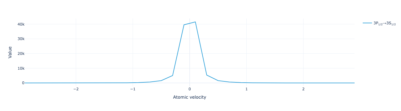

Plot the real and imaginary parts of the density-matrix elements for each velocity bin:

sol.visualize()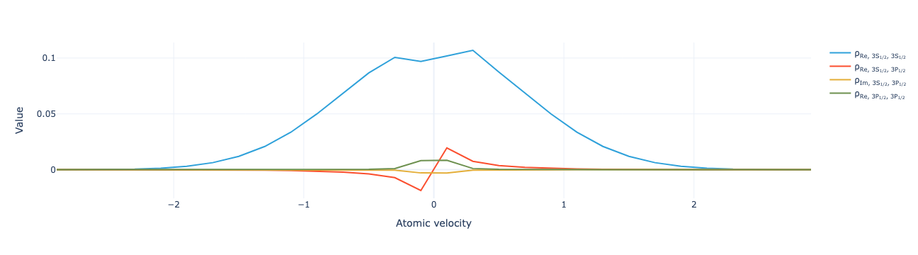

Plot just the level populations:

model.level_population(sol).visualize()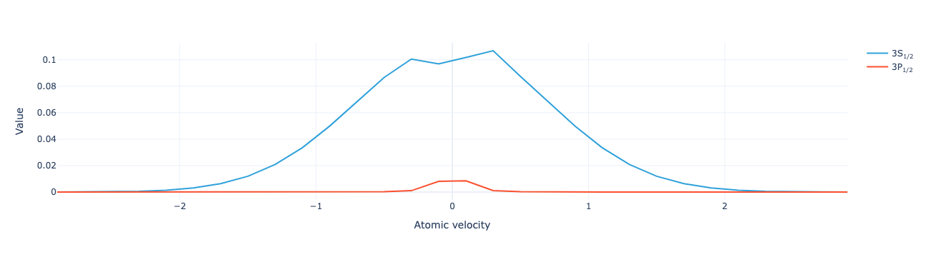

Plot the total atomic population:

model.population(sol).visualize()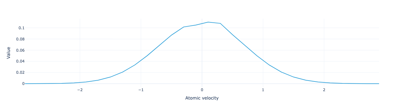

Note that the above visualizations plot the contribution to the quantity from each velocity group. If the velocity groups are not all of the same width, this will cause the plots to appear distorted. In this case one can instead plot the velocity distribution of the quantities using flux_distribution, population_distribution, etc. To plot the velocity distribution of the density-matrix elements, use velocity_normalize(sol).

Table 1: Operators that can be applied to the solution of an LGS model

	Description
population	Fraction of total atomic population in each velocity group
total_population	Total atomic population (should equal 1)
population_distribution	Atomic population per unit velocity interval
level_population	Population of each atomic level in each velocity group
total_level_population	Total atomic population in each level
level_population_distribution	Level population per unit velocity interval
flux	Return flux on each transition from each velocity group
total_flux	Total return flux
flux_distribution	Return flux per unit velocity interval
velocity_sum	Sum over velocity groups
velocity_normalize	Normalize by velocity-group width

Check that the atomic population summed over all velocity groups is approximately 1:

model.total_population(sol).item()

0.9933937631461671

type(to_matrix(model.operator.assemble(Mu({'IntensitySI1': 1e3}))))

scipy.sparse._csr.csr_array

---

LGSSystem.adaptive_stationary_model

def adaptive_stationary_model(
    mu, # Parameter values to use during velocity-group refinement
    vg:int=6, # Initial velocity groups
    max_weight:float=0.01, # Maximum fraction of the return flux from any one velocity group
)->StationaryModel: # Steady-state LGS model with more velocity groups in regions that produce more return flux

Create a StationaryModel with narrower velocity bins in velocity regions with higher flux.

Create a model with adaptively refined velocity groups using a particular value for the intensity parameter during refinement:

model = lgs.adaptive_stationary_model({'IntensitySI1': 1e3}, max_weight=0.2)

Solve and find total flux:

model.total_flux({'IntensitySI1': 1e3}).item()

137701.2731471721

Solve for the density matrix. The solution has density-matrix values for 17 velocity groups:

sol = model.solve({'IntensitySI1': 1e3})
sol

∅ ⛒ Atomic velocity(16) ⛒ Density matrix(4)

<xarray.DataArray (Atomic velocity: 16, Density matrix: 4)> Size: 512B
array([[ 0.0023 ,  -2e-05 , -1.2e-07,  3.8e-07],
       [  0.076 , -0.0011 , -1.1e-05,  3.2e-05],
       [  0.16  , -0.0046 , -9.3e-05,  0.00027],
       [  0.12  , -0.0068 , -0.00028,  0.00079],
       [  0.064 , -0.0071 , -0.00058,  0.0017 ],
       [  0.028 , -0.0056 , -0.00092,  0.0026 ],
       [  0.009 , -0.0027 , -0.00088,  0.0025 ],
       [  0.006 , -0.0014 , -0.0014 ,   0.004 ],
       [ 0.0075 ,  0.0018 , -0.0018 ,   0.005 ],
       [  0.016 ,  0.0048 , -0.0016 ,  0.0044 ],
       [  0.043 ,  0.0087 , -0.0014 ,   0.004 ],
       [  0.073 ,  0.0081 , -0.00067,  0.0019 ],
       [  0.12  ,  0.0069 , -0.00028,  0.00081],
       [  0.16  ,  0.0046 , -9.4e-05,  0.00027],
       [  0.076 ,  0.0011 , -1.1e-05,  3.2e-05],
       [ 0.0023 ,   2e-05 , -1.2e-07,  3.8e-07]])
Coordinates:
  * Atomic velocity  (Atomic velocity) float64 128B -2.5 -1.5 -0.75 ... 1.5 2.5
  * Density matrix   (Density matrix) <U50 800B 'ρ<sub>Re, 3S<sub>1/2</sub>, ...

xarray.DataArray

• Atomic velocity: 16
• Density matrix: 4

• 0.002312 -1.985e-05 -1.218e-07 ... 1.99e-05 -1.221e-07 3.779e-07

  array([[ 0.0023 ,  -2e-05 , -1.2e-07,  3.8e-07],
         [  0.076 , -0.0011 , -1.1e-05,  3.2e-05],
         [  0.16  , -0.0046 , -9.3e-05,  0.00027],
         [  0.12  , -0.0068 , -0.00028,  0.00079],
         [  0.064 , -0.0071 , -0.00058,  0.0017 ],
         [  0.028 , -0.0056 , -0.00092,  0.0026 ],
         [  0.009 , -0.0027 , -0.00088,  0.0025 ],
         [  0.006 , -0.0014 , -0.0014 ,   0.004 ],
         [ 0.0075 ,  0.0018 , -0.0018 ,   0.005 ],
         [  0.016 ,  0.0048 , -0.0016 ,  0.0044 ],
         [  0.043 ,  0.0087 , -0.0014 ,   0.004 ],
         [  0.073 ,  0.0081 , -0.00067,  0.0019 ],
         [  0.12  ,  0.0069 , -0.00028,  0.00081],
         [  0.16  ,  0.0046 , -9.4e-05,  0.00027],
         [  0.076 ,  0.0011 , -1.1e-05,  3.2e-05],
         [ 0.0023 ,   2e-05 , -1.2e-07,  3.8e-07]])

• Coordinates: (2)
  • Atomic velocity
    (Atomic velocity)
    float64
    -2.5 -1.5 -0.75 ... 0.75 1.5 2.5

    array([-2.5     , -1.5     , -0.75    , -0.375   , -0.1875  , -0.09375 ,
           -0.046875, -0.015625,  0.015625,  0.046875,  0.09375 ,  0.1875  ,
            0.375   ,  0.75    ,  1.5     ,  2.5     ])

  • Density matrix
    (Density matrix)
    <U50
    'ρ<sub>Re, 3S_1/2, 3S<...

    array(['ρ<sub>Re, 3S<sub>1/2</sub>, 3S<sub>1/2</sub></sub>',
           'ρ<sub>Re, 3S<sub>1/2</sub>, 3P<sub>1/2</sub></sub>',
           'ρ<sub>Im, 3S<sub>1/2</sub>, 3P<sub>1/2</sub></sub>',
           'ρ<sub>Re, 3P<sub>1/2</sub>, 3P<sub>1/2</sub></sub>'], dtype='<U50')

Plot the velocity distribution of flux. Each point marks the center of a velocity group:

model.flux_distribution(sol).visualize(markers=True)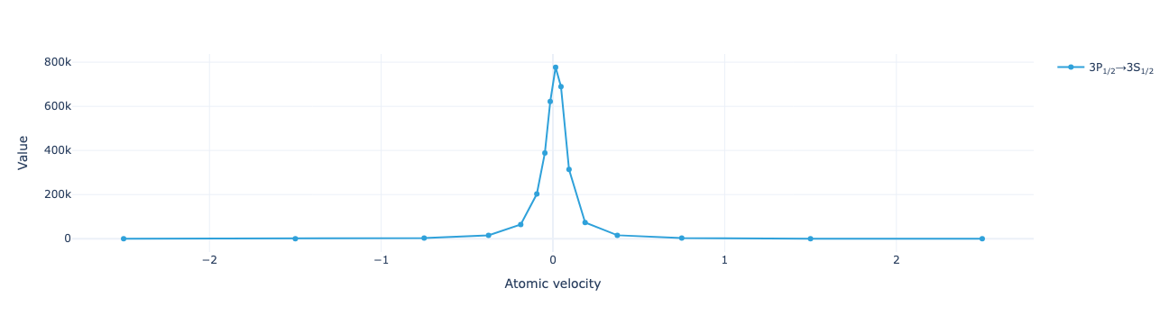

Velocity distribution of the density matrix:

model.velocity_normalize(sol).visualize()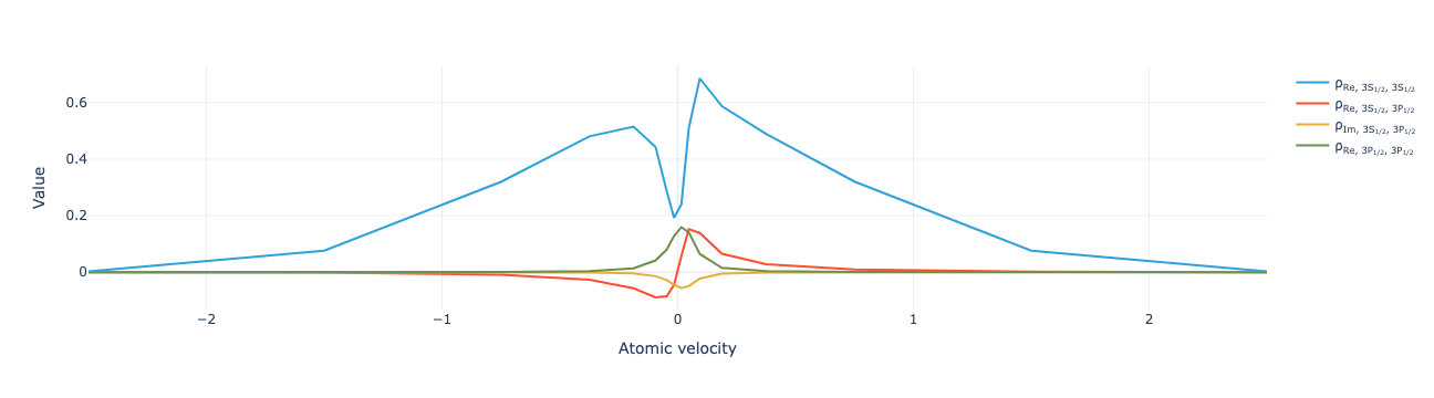

Of the total population:

model.population_distribution(sol).visualize()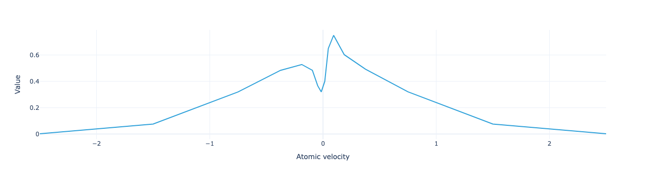

Of the level populations:

model.level_population_distribution(sol).visualize()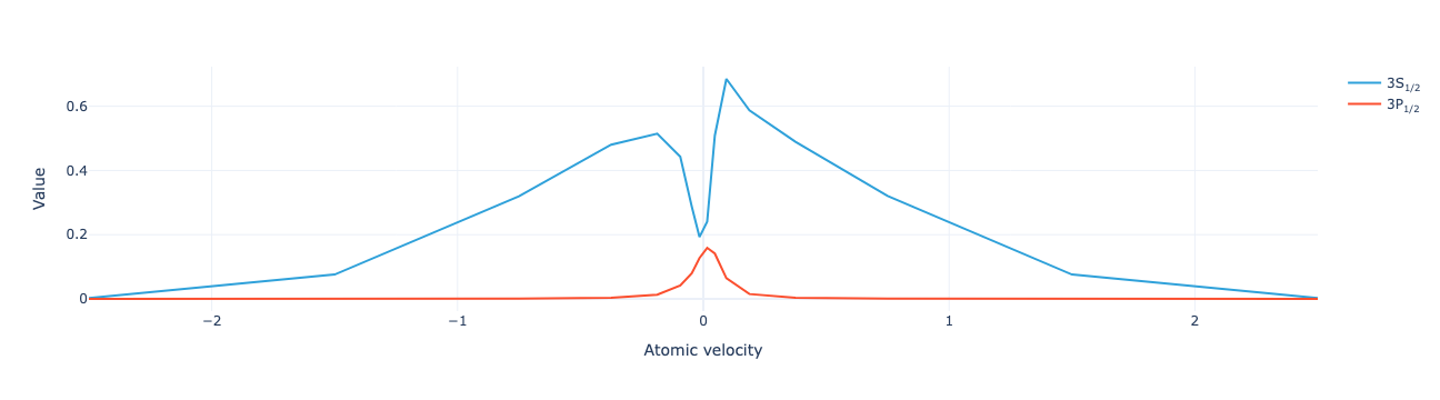

---

LGSSystem.instationary_model

def instationary_model(
    vg:Union=6, # Specification of velocity groups
    T:float=1e-06, # Final time (seconds)
    num_values:int=100, # Number of time step values to return
    initial_rho:NoneType=None, # Initial density matrix. `None` means to use the thermal distribution
    time_stepper:BDFTimeStepper=BDFTimeStepper(), # Solver to use
)->InstationaryModel: # Model for the LGS system dynamics

Create an InstationaryModel for the LGS system dynamics.

An instationary model with 30 velocity groups:

vg=30
num_values=100
T=1.e-4
inst_model = lgs.instationary_model(
    vg=vg, 
    T=T, 
    num_values=num_values
)

The BDF solver is efficient but can be very sensitive to the absolute and relative tolerance values. Set appropriate values for this problem:

pymor.basic.set_defaults({
    'pylgs.pymor.timestepping.cvode_solver_options.cvode_bdf_atol': 1e-3,
    'pylgs.pymor.timestepping.cvode_solver_options.cvode_bdf_rtol': 1e-6
})

Solve for a constant value of intensity:

inst_sol = inst_model.solve({'IntensitySI1': 1e3})

Visualize the total flux as a function of time:

inst_model.total_population(inst_sol).visualize()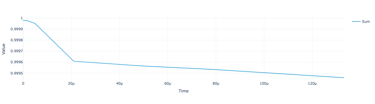

inst_model.total_flux(inst_sol).visualize()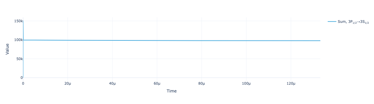

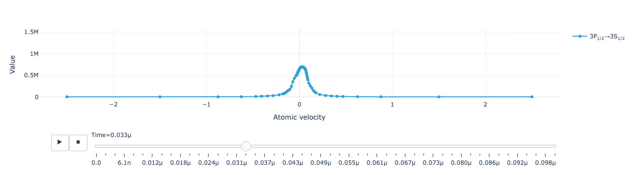
Plot the density matrix elements as a function of atomic velocity and animate as a function of time:

inst_model.velocity_normalize(inst_sol).visualize().update_layout(sliders=[dict(active=4)])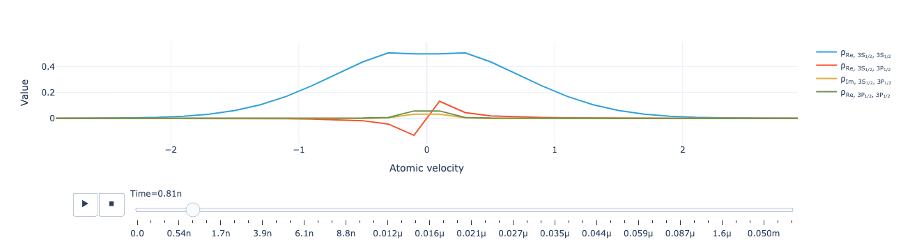

Animate the population distribution as a function of time:

inst_model.population_distribution(inst_sol).visualize()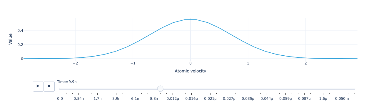

Animate the level population distributions:

inst_model.level_population_distribution(inst_sol).visualize()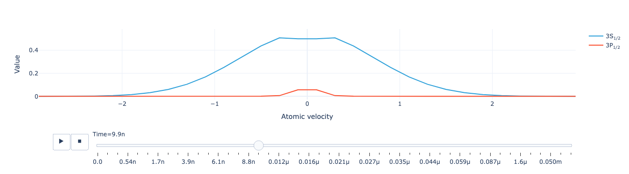

Set a shorter evolution time for the model:

T=1e-7
num_values=50

inst_model = inst_model.with_(T=T, num_values=num_values)

Solve the model with a modulated intensity parameter:

inst_mu = {'IntensitySI1': "5000.*sin(1.e8*t)**2"}

pymor.basic.set_defaults({
    'pylgs.pymor.timestepping.cvode_solver_options.cvode_bdf_atol': 3e-4,
    'pylgs.pymor.timestepping.cvode_solver_options.cvode_bdf_rtol': 1e-7
})

inst_sol = inst_model.solve(inst_mu)

Visualize the total flux as a function of time:

inst_plot = inst_model.total_flux(inst_sol).visualize()
inst_plot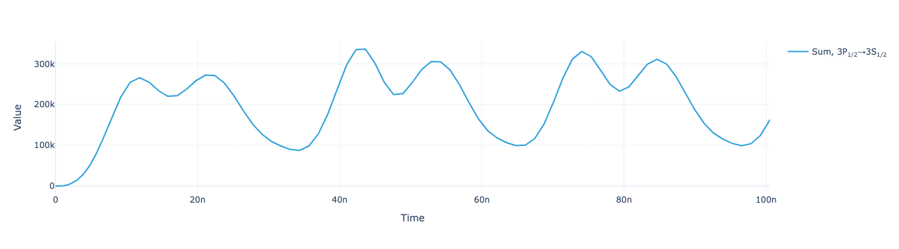

Visualize the density matrix elements:

inst_model.velocity_normalize(inst_sol).visualize()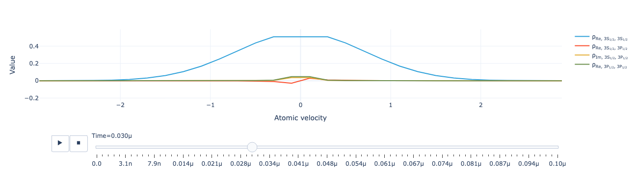

Visualize the flux distribution:

inst_model.flux_distribution(inst_sol).visualize()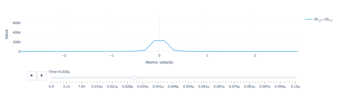

inst_model.population_distribution(inst_sol).visualize()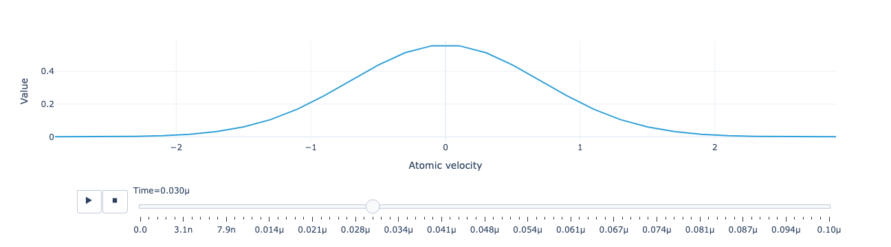

numpy_instationary_model

The numpy model is currently much faster for explicit methods than the xarray model. However, it requires Kronecker-expanding the DM x VG product-space operators. It might be a little faster if this wasn’t necessary, but no more than a factor of 2 or 3. It seems like BlockOperator and BlockVectorArray are designed for this, but it looks like they are not optimized for speed. It could be implemented by optimizing XarrayMatrixOperator so that all apply operations can bypass xarray and use numpy instead. Note that sparse DataArrays currently use COO format, would want to switch to CSR, but need to enforce 2D matrices or allow N-D CSR arrays.

Evaluating the coefficients at a given time also could be sped up a little (use lambdify to convert ExpressionFunctions to GenericFunctions), but it is not the dominant source of computation time.

# def to_dense_matrix(op):
#     a = to_matrix(op)
#     try: a = a.todense()
#     except: pass
#     return a

---

LGSSystem.numpy_instationary_model

def numpy_instationary_model(
    vg, T:float=1e-06, # Final time (seconds)
    num_values:int=100, # Number of time step values to return
    initial_rho:NoneType=None, # Initial density matrix. `None` means to use the thermal distribution
    time_stepper:BDFTimeStepper=BDFTimeStepper(), # Solver to use
): # Model for the LGS system dynamics

npin_model = lgs.numpy_instationary_model(
    vg=vg, 
    T=T, 
    num_values=num_values,
    time_stepper=AdamsTimeStepper()
)

Solve the model with a modulated intensity parameter:

npin_sol = npin_model.output(inst_mu)

plt.plot(npin_sol.sum(0));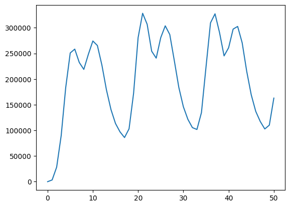

plt.plot(inst_model.total_flux(inst_sol).to_numpy()[0]);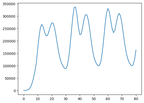

plt.plot(npin_sol.T);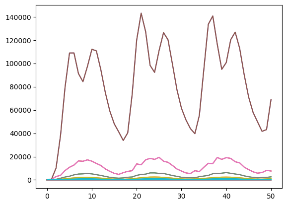

plt.plot(npin_sol.sum(1));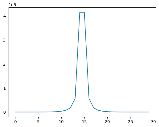

---

LGSSystem.stationary_floquet_model

def stationary_floquet_model(
    mu, # Parameter specification for parameters modulated at a frequency `nu`
    time, # List of time values to use for reconstruction
    n_vector, # Number of terms in the system Fourier series
    nu:str='nu', # Name of the frequency variable
    n_operator:NoneType=None, # Number of terms in the operator Fourier series. `None` defaults to `n_vector` - 1
    vg:Union=6, # Specification of velocity groups
    solver:NoneType=None
)->StationaryFloquetModel: # Model for the Fourier coefficients of the periodic LGS system

Return a StationaryFloquetModel for the Fourier coefficients of the periodic state of a modulated LGS system.

The StationaryFloquetModel solves for the periodic state of a modulated system after the transient dynamics have died out.

Build a stationary Floquet model for six Fourier harmonics of a system with sinusoidally modulated intensity:

floq_model = lgs.stationary_floquet_model(
    mu={'IntensitySI1': "5000.*sin(nu*t)**2"},
    time=np.linspace(0, T, num_values),
    n_vector=10,
    vg=vg
)

Define values for the modulation frequency and light detuning:

Solve for the periodic state. The solution contains 7 Fourier coefficients for each density-matrix element in each velocity group:

floq_mu = Mu(nu=1e8)

floq_sol = floq_model.solve(floq_mu)

floq_sol = floq_model.solve(floq_mu)

CPU times: user 29.6 ms, sys: 4.41 ms, total: 34 ms
Wall time: 32.9 ms

floq_plot = floq_model.reconstructed_total_flux(floq_sol, floq_mu).real.visualize()
floq_plot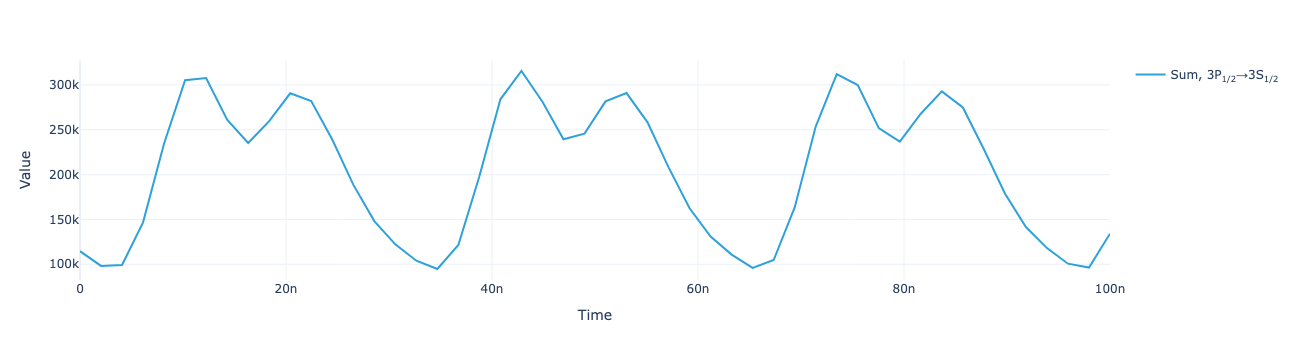

floq_plot = floq_model.flux_distribution(floq_sol, floq_mu).real.visualize()
floq_plot

floq_plot = floq_model.reconstructed_flux_distribution(floq_sol, floq_mu).real.visualize()
floq_plot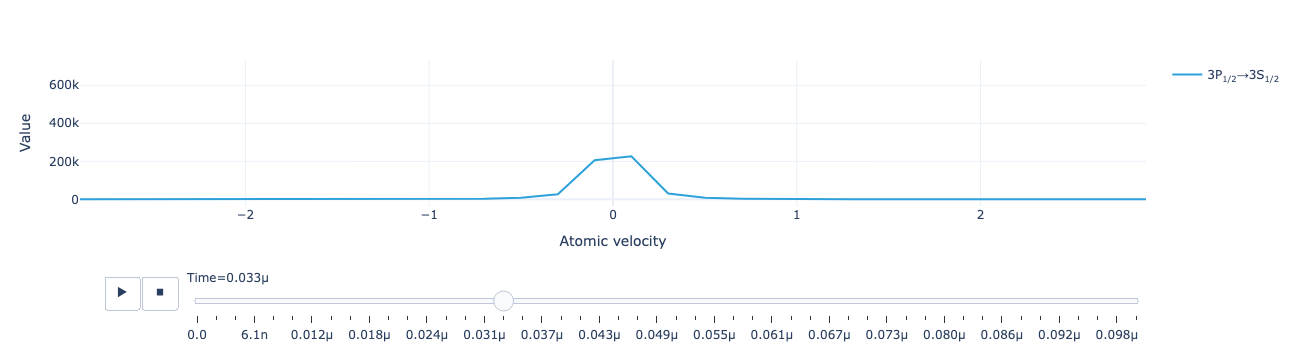

floq_model.reconstructed_flux_distribution(floq_sol, floq_mu).real.array.sum(['Time', 'Transition'])

<xarray.DataArray (Atomic velocity: 30)> Size: 240B
array([   9.2  ,  3.2e+01,   1e+02 ,  3.2e+02,   9e+02 ,  2.4e+03,  6.2e+03,  1.5e+04,  3.4e+04,  7.7e+04,  1.7e+05,  3.8e+05,  9.4e+05,
        2.9e+06,   2e+07 ,  2.2e+07,  3.3e+06,  9.6e+05,  3.8e+05,  1.7e+05,  7.7e+04,  3.4e+04,  1.5e+04,  6.2e+03,  2.4e+03,  9.1e+02,
        3.2e+02,   1e+02 ,  3.2e+01,    9.3  ])
Coordinates:
  * Atomic velocity  (Atomic velocity) float64 240B -2.9 -2.7 -2.5 ... 2.7 2.9

xarray.DataArray

• Atomic velocity: 30

• 9.25 32.15 104.4 317.3 904.9 ... 905.8 317.6 104.5 32.17 9.257

  array([   9.2  ,  3.2e+01,   1e+02 ,  3.2e+02,   9e+02 ,  2.4e+03,  6.2e+03,  1.5e+04,  3.4e+04,  7.7e+04,  1.7e+05,  3.8e+05,  9.4e+05,
          2.9e+06,   2e+07 ,  2.2e+07,  3.3e+06,  9.6e+05,  3.8e+05,  1.7e+05,  7.7e+04,  3.4e+04,  1.5e+04,  6.2e+03,  2.4e+03,  9.1e+02,
          3.2e+02,   1e+02 ,  3.2e+01,    9.3  ])

• Coordinates: (1)
  • Atomic velocity
    (Atomic velocity)
    float64
    -2.9 -2.7 -2.5 -2.3 ... 2.5 2.7 2.9

    array([-2.9, -2.7, -2.5, -2.3, -2.1, -1.9, -1.7, -1.5, -1.3, -1.1, -0.9, -0.7,
           -0.5, -0.3, -0.1,  0.1,  0.3,  0.5,  0.7,  0.9,  1.1,  1.3,  1.5,  1.7,
            1.9,  2.1,  2.3,  2.5,  2.7,  2.9])

import plotly.graph_objects as go

go.Figure(data=[floq_plot.data[0], inst_plot.data[0],])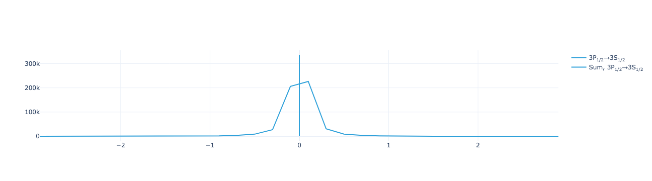

The real and imaginary parts of the Fourier coefficients of the time-dependent return flux:

floq_model.total_flux(floq_sol).real.visualize()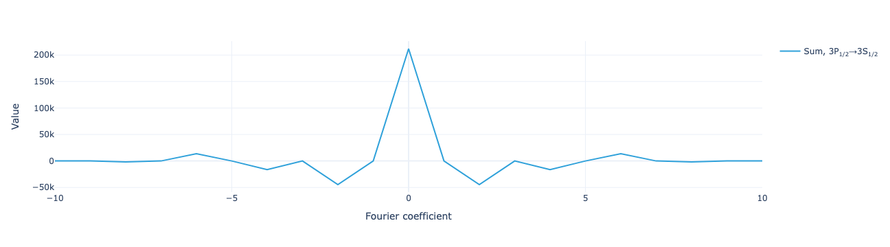

floq_model.reconstruct(floq_sol, floq_mu).visualize()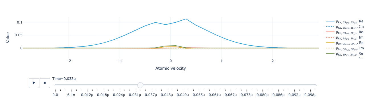

The total return flux reconstructed as a function of time:

The real and imaginary parts of the Fourier coefficients of the real and imaginary parts of the density-matrix elements:

floq_model.velocity_normalize(floq_mu).visualize()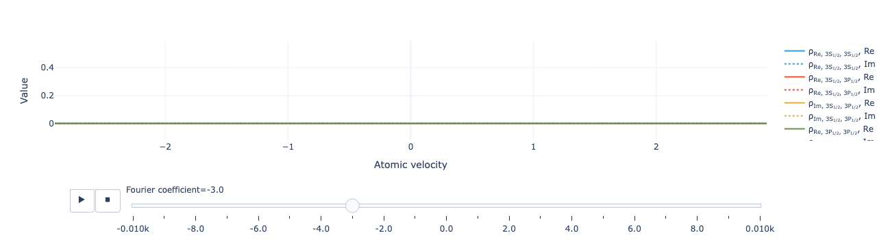

The real and imaginary parts of the density-matrix elements reconstructed as a function of time:

floq_model.velocity_normalize(floq_model.reconstruct(floq_sol, floq_mu)).real.visualize()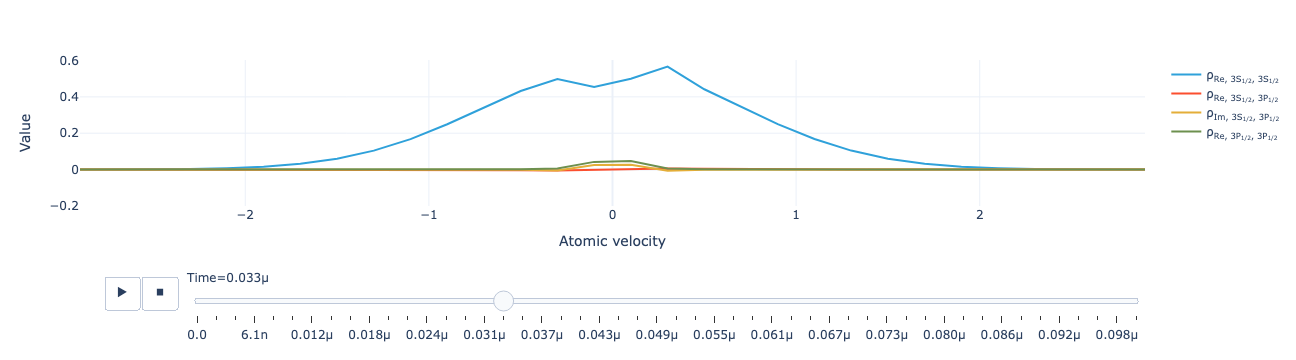

---

LGSSystem.adaptive_stationary_floquet_model

def adaptive_stationary_floquet_model(
    mu, # Parameter specification for parameters modulated at a frequency `nu`
    mu_refine, time, # List of time values to use for reconstruction
    n_vector, # Number of terms in the system Fourier series
    nu:str='nu', # Name of the frequency variable
    n_operator:NoneType=None, # Number of terms in the operator Fourier series. `None` defaults to `n_vector` - 1
    vg:int=6, # Initial velocity groups
    solver:NoneType=None, max_weight:float=0.01, # Maximum fraction of the return flux from any one velocity group
    subdivisions:int=4
)->StationaryFloquetModel: # Steady-state LGS model with more velocity groups in regions that produce more return flux

Create a StationaryModel with narrower velocity bins in velocity regions with higher flux.

Create a model with adaptively refined velocity groups using a particular value for the intensity parameter during refinement:

mu = {'nu': 1e8}
model, sol = lgs.adaptive_stationary_floquet_model(
    mu={'IntensitySI1': "5000.*sin(nu*t)**2"},
    mu_refine=mu,
    time=np.linspace(0, T, num_values),
    n_vector=20,
    max_weight=0.05
)

Creating model with 6 velocity groups
Solving model
Creating model with 12 velocity groups
Solving model
Creating model with 24 velocity groups
Solving model
Creating model with 42 velocity groups
Solving model
Creating model with 66 velocity groups
Solving model

model.reconstructed_total_flux(sol, mu).real.visualize()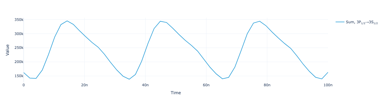

model.reconstructed_flux_distribution(sol, mu).real.visualize(markers=True)