from pylgs.all import *Polychromatic LGS
A multi-level sodium system excited by 330 nm light
Define a LGS system pumped by 330 nm light:
lgs = LGSSystem(
    'Na330',
    {
        'IntensitySI1': 5000.,
        'BFieldG': 0.5,
        'EllipticityDegrees1': 45.,
        'PolarizationAngleDegrees1': 0,
        'DetuningHz1': 1.0832e9,
        'LaserWidthHz1': 10.0e6,
        'MagneticZenithDegrees': 45.,
        'MagneticAzimuthDegrees': 45.,
        'SDampingCollisionRatePerS': 4081.63,
        'BeamTransitRatePerS': 131.944,
        'VccRatePerS': 28571.,
        'TemperatureK': 185.,
        'RecoilParameter': 1.
    }
)
The system is made up of 774 density-matrix elements describing 7 atomic levels:
lgs.level_population.rangeLevel(7)
<xarray.DataArray 'XarrayVectorSpace' (Level: 7)> Size: 56B
array([0., 0., 0., 0., 0., 0., 0.])
Coordinates:
  * Level    (Level) <U16 448B '3D<sub>3/2</sub>' ... '3P<sub>1/2</sub>'
HTML(', '.join(lgs.level_population.range.coords['Level'].data))
3D3/2, 4P3/2, 3D5/2, 3P3/2, 4S1/2, 3S1/2, 3P1/2
Steady-state model
Adaptively refine velocity groups
Build a steady-state model with adaptively refined velocity groups:
model = lgs.adaptive_stationary_model({}, max_weight=0.02)Solve for the density matrix. There are 77 velocity groups in the model:
sol = model.solve()
sol
∅ ⛒ Atomic velocity(77) ⛒ Density matrix(774)
<xarray.DataArray (Atomic velocity: 77, Density matrix: 774)> Size: 477kB
array([[ 4.81176178e-04,  5.34383694e-05, -5.34345398e-05, ...,
        -7.62458011e-08, -1.59213581e-10,  4.80993663e-10],
       [ 1.57798955e-02,  1.75251498e-03, -1.75236074e-03, ...,
        -4.16181537e-06, -1.44907597e-08,  3.47742328e-08],
       [ 1.36170875e-02,  1.51285607e-03, -1.51264792e-03, ...,
        -6.12657935e-06, -3.65981137e-08,  7.93941184e-08],
       ...,
       [ 3.46659562e-04,  4.29832767e-05, -4.25355464e-05, ...,
         1.13082229e-07, -3.42890749e-10,  8.25194594e-10],
       [ 8.73280729e-04,  1.00106012e-04, -9.98470213e-05, ...,
         2.02082796e-07, -5.61752597e-10,  1.43885993e-09],
       [ 4.79681482e-04,  5.35790217e-05, -5.35574066e-05, ...,
         7.67512540e-08, -1.60052771e-10,  4.82713824e-10]],
      shape=(77, 774))
Coordinates:
  * Atomic velocity  (Atomic velocity) float64 616B -2.5 -1.5 ... 1.875 2.5
* Density matrix (Density matrix) <U68 211kB 'ρ<sub>Re, (3S<sub>1/2</sub>...Plot the total return flux for each transition as a bar chart:
model.total_flux(sol).visualize()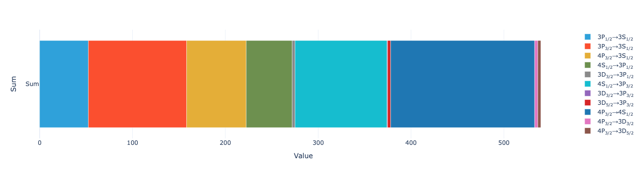
Plot the flux as a function of velocity:
model.flux_distribution(sol).visualize(xaxis_range=(-1, 2))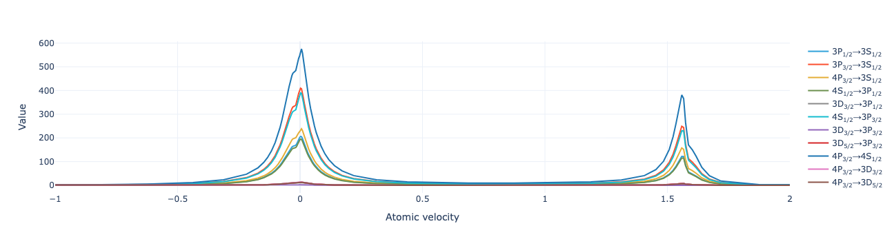
model.flux_distribution(sol).visualize(xaxis_range=(-1, 2))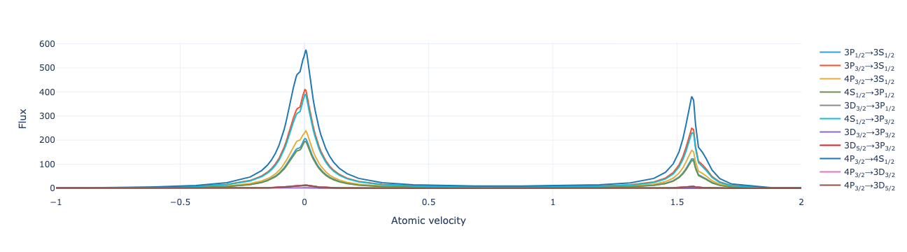
Transient dynamics model
Build a model for the transient dynamics:
model = lgs.instationary_model(
    vg=model.data['velocity_groups'],
    T=1e-6,
    num_values=101
)
Set tolerances for the BDF solver:
pymor.basic.set_defaults({
    'pylgs.pymor.timestepping.cvode_solver_options.cvode_bdf_atol': 1e-6,
    'pylgs.pymor.timestepping.cvode_solver_options.cvode_bdf_rtol': 1e-5,
})
Solve for the density matrix as a function of time:
sol = model.solve()solTime(48) ⛒ Atomic velocity(77) ⛒ Density matrix(774)
<xarray.DataArray (Time: 48, Atomic velocity: 77, Density matrix: 774)> Size: 23MB
array([[[ 2.90977780e-04,  0.00000000e+00,  0.00000000e+00, ...,
          0.00000000e+00,  0.00000000e+00,  0.00000000e+00],
        [ 9.53884200e-03,  0.00000000e+00,  0.00000000e+00, ...,
          0.00000000e+00,  0.00000000e+00,  0.00000000e+00],
        [ 8.22157246e-03,  0.00000000e+00,  0.00000000e+00, ...,
          0.00000000e+00,  0.00000000e+00,  0.00000000e+00],
        ...,
        [ 2.30122164e-04,  0.00000000e+00,  0.00000000e+00, ...,
          0.00000000e+00,  0.00000000e+00,  0.00000000e+00],
        [ 5.40662112e-04,  0.00000000e+00,  0.00000000e+00, ...,
          0.00000000e+00,  0.00000000e+00,  0.00000000e+00],
        [ 2.90977780e-04,  0.00000000e+00,  0.00000000e+00, ...,
          0.00000000e+00,  0.00000000e+00,  0.00000000e+00]],

       [[ 2.90977780e-04,  0.00000000e+00,  0.00000000e+00, ...,
         -2.01285531e-14, -5.79463896e-11,  2.30793494e-17],
        [ 9.53884200e-03,  0.00000000e+00,  0.00000000e+00, ...,
         -3.95739321e-13, -1.89960022e-09,  7.56587900e-16],
        [ 8.22157246e-03,  0.00000000e+00,  0.00000000e+00, ...,
         -1.98813085e-13, -1.63727430e-09,  6.52106644e-16],
...
          1.92070767e-07, -5.82489819e-10,  2.18970406e-09],
        [ 5.40356997e-04,  1.99644086e-07,  5.15788552e-08, ...,
          4.12741922e-07, -1.14739043e-09,  4.69286751e-09],
        [ 2.91009975e-04,  2.46249542e-08,  5.26512628e-09, ...,
          1.66544953e-07, -3.47304600e-10,  1.97236720e-09]],

       [[ 2.91066612e-04,  2.99523228e-08, -2.59348021e-09, ...,
         -1.66718407e-07, -3.48121939e-10,  1.77222676e-09],
        [ 9.54197122e-03,  1.01752190e-06, -1.14974508e-07, ...,
         -9.11224032e-06, -3.17257246e-08,  1.00073073e-07],
        [ 8.22501861e-03,  1.05059828e-06, -8.63273167e-08, ...,
         -1.34707937e-05, -8.04639253e-08,  1.95221527e-07],
        ...,
        [ 2.29222925e-04,  5.26935391e-07,  5.61885394e-08, ...,
          1.92369176e-07, -5.83396090e-10,  2.03285350e-09],
        [ 5.40272560e-04,  3.13699724e-07,  2.23127567e-08, ...,
          4.12813932e-07, -1.14758955e-09,  4.31984715e-09],
        [ 2.91035094e-04,  4.34481998e-08, -1.21067812e-09, ...,
          1.66516368e-07, -3.47244310e-10,  1.77041703e-09]]],
      shape=(48, 77, 774))
Coordinates:
  * Time             (Time) float64 384B 0.0 1.999e-14 ... 8.079e-07 1.161e-06
  * Atomic velocity  (Atomic velocity) float64 616B -2.5 -1.5 ... 1.875 2.5
* Density matrix (Density matrix) <U68 211kB 'ρ<sub>Re, (3S<sub>1/2</sub>...Plot the return flux for each transition:
model.total_flux(sol).visualize()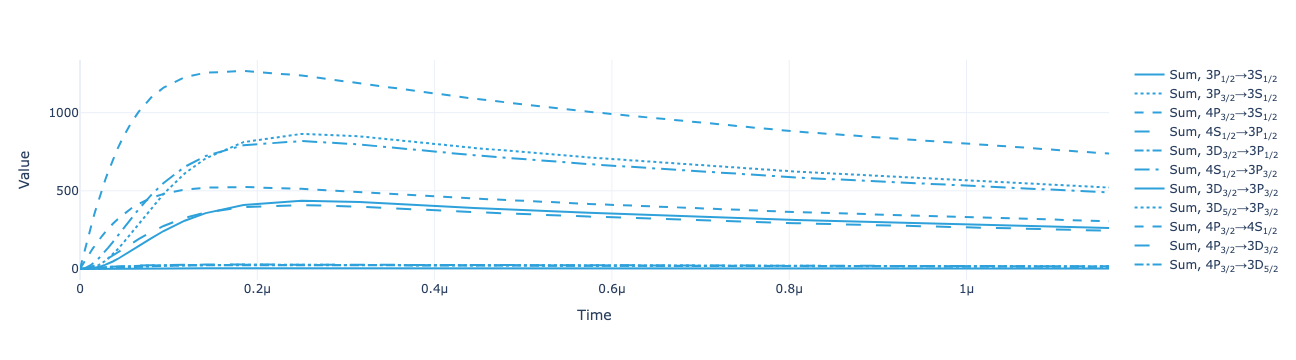
model.total_flux(sol).visualize()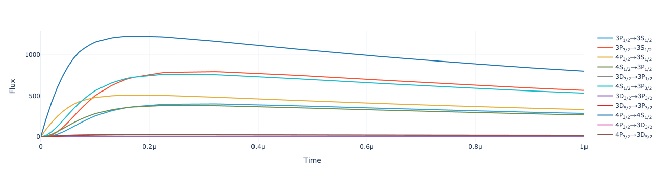
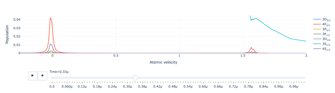
Animate the level population distribution as a function of time:
model.level_population_distribution(sol).visualize(xaxis_range=(-.25, 2), yaxis_range=(0, .045))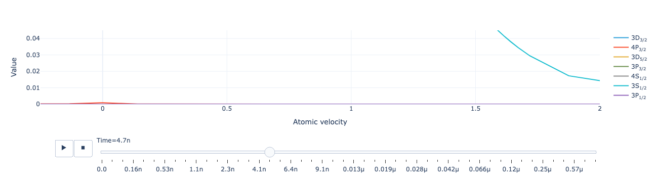
model.level_population_distribution(sol).visualize(xaxis_range=(-.25, 2), yaxis_range=(0, .045))