from pylgs.all import *
import numpy as np
import pymorSodium LGS
Simulate a sodium LGS beacon
Imports
System setup
Define an LGS system on the D\(_2\) line with pump and repump beams, with all parameters fixed except for the light intensities and the magnetic-field strength:
lgs = LGSSystem(
    'NaD2_Repump',
    {
        'EllipticityDegrees1': 45.,
        'PolarizationAngleDegrees1': 0,
        'DetuningHz1': 1.0832e9,
        'LaserWidthHz1': 10.0e6,
        'EllipticityDegrees2': 45.,
        'PolarizationAngleDegrees2': 0,
        'DetuningHz2': -6.268e8,
        'LaserWidthHz2': 10.0e6,
        'MagneticZenithDegrees': 45.,
        'MagneticAzimuthDegrees': 45.,
        'SDampingCollisionRatePerS': 4081.63,
        'BeamTransitRatePerS': 131.944,
        'VccRatePerS': 28571.,
        'TemperatureK': 185.,
        'RecoilParameter': 1
    }
)
The model contains equations for 374 density-matrix elements:
lgs.A_ind.rangeDensity matrix(374)
<xarray.DataArray 'XarrayVectorSpace' (Density matrix: 374)> Size: 3kB
array([0., 0., 0., 0., 0., 0., 0., 0., 0., 0., 0., 0., 0., 0., 0., 0., 0.,
       0., 0., 0., 0., 0., 0., 0., 0., 0., 0., 0., 0., 0., 0., 0., 0., 0.,
       0., 0., 0., 0., 0., 0., 0., 0., 0., 0., 0., 0., 0., 0., 0., 0., 0.,
       0., 0., 0., 0., 0., 0., 0., 0., 0., 0., 0., 0., 0., 0., 0., 0., 0.,
       0., 0., 0., 0., 0., 0., 0., 0., 0., 0., 0., 0., 0., 0., 0., 0., 0.,
       0., 0., 0., 0., 0., 0., 0., 0., 0., 0., 0., 0., 0., 0., 0., 0., 0.,
       0., 0., 0., 0., 0., 0., 0., 0., 0., 0., 0., 0., 0., 0., 0., 0., 0.,
       0., 0., 0., 0., 0., 0., 0., 0., 0., 0., 0., 0., 0., 0., 0., 0., 0.,
       0., 0., 0., 0., 0., 0., 0., 0., 0., 0., 0., 0., 0., 0., 0., 0., 0.,
       0., 0., 0., 0., 0., 0., 0., 0., 0., 0., 0., 0., 0., 0., 0., 0., 0.,
       0., 0., 0., 0., 0., 0., 0., 0., 0., 0., 0., 0., 0., 0., 0., 0., 0.,
       0., 0., 0., 0., 0., 0., 0., 0., 0., 0., 0., 0., 0., 0., 0., 0., 0.,
       0., 0., 0., 0., 0., 0., 0., 0., 0., 0., 0., 0., 0., 0., 0., 0., 0.,
       0., 0., 0., 0., 0., 0., 0., 0., 0., 0., 0., 0., 0., 0., 0., 0., 0.,
       0., 0., 0., 0., 0., 0., 0., 0., 0., 0., 0., 0., 0., 0., 0., 0., 0.,
       0., 0., 0., 0., 0., 0., 0., 0., 0., 0., 0., 0., 0., 0., 0., 0., 0.,
       0., 0., 0., 0., 0., 0., 0., 0., 0., 0., 0., 0., 0., 0., 0., 0., 0.,
       0., 0., 0., 0., 0., 0., 0., 0., 0., 0., 0., 0., 0., 0., 0., 0., 0.,
       0., 0., 0., 0., 0., 0., 0., 0., 0., 0., 0., 0., 0., 0., 0., 0., 0.,
       0., 0., 0., 0., 0., 0., 0., 0., 0., 0., 0., 0., 0., 0., 0., 0., 0.,
       0., 0., 0., 0., 0., 0., 0., 0., 0., 0., 0., 0., 0., 0., 0., 0., 0.,
       0., 0., 0., 0., 0., 0., 0., 0., 0., 0., 0., 0., 0., 0., 0., 0., 0.])
Coordinates:
* Density matrix (Density matrix) <U68 102kB 'ρ<sub>Re, (3S<sub>1/2</sub>,...Define sample values for the variable parameters:
params = {'IntensitySI1': 5., 'IntensitySI2': 46., 'BFieldG': 0.5}Steady state of a cw LGS
Evenly spaced velocity groups
Build a model for the steady state of a cw LGS with 200 evenly spaced velocity groups:
model = lgs.stationary_model(vg=200)Find the steady-state return flux:
model.total_flux(params).item()13625.270170636119Find the density matrix for each of the 200 velocity groups:
sol = model.solve(params)
sol
∅ ⛒ Atomic velocity(200) ⛒ Density matrix(374)
<xarray.DataArray (Atomic velocity: 200, Density matrix: 374)> Size: 598kB
array([[ 4.39820983e-07,  1.36790151e-07, -1.36692295e-07, ...,
         4.11349074e-11,  2.15032835e-13,  3.90993997e-14],
       [ 5.25623812e-07,  1.63475921e-07, -1.63358568e-07, ...,
         4.96457648e-11,  2.62098979e-13,  4.73161241e-14],
       [ 6.27016972e-07,  1.95009268e-07, -1.94868907e-07, ...,
         5.98154460e-11,  3.18954045e-13,  5.71688763e-14],
       ...,
       [ 6.25164290e-07,  1.95204688e-07, -1.95037855e-07, ...,
        -6.26906842e-11,  3.50162743e-13,  6.07662718e-14],
       [ 5.24087250e-07,  1.63638185e-07, -1.63498884e-07, ...,
        -5.20072715e-11,  2.87471429e-13,  5.02407809e-14],
       [ 4.38562258e-07,  1.36929696e-07, -1.36813582e-07, ...,
        -4.30715577e-11,  2.35630651e-13,  4.14737939e-14]],
      shape=(200, 374))
Coordinates:
  * Atomic velocity  (Atomic velocity) float64 2kB -2.985 -2.955 ... 2.955 2.985
* Density matrix (Density matrix) <U68 102kB 'ρ<sub>Re, (3S<sub>1/2</sub>...The result is expressed as an XarrayVectorArray object representing 200 vectors each of size 374. The XarrayVectorArray is a wrapper for an xarray DataArray, which can be accessed via the XarrayVectorArray.array attribute:
sol.array<xarray.DataArray (Atomic velocity: 200, Density matrix: 374)> Size: 598kB
array([[ 4.39820983e-07,  1.36790151e-07, -1.36692295e-07, ...,
         4.11349074e-11,  2.15032835e-13,  3.90993997e-14],
       [ 5.25623812e-07,  1.63475921e-07, -1.63358568e-07, ...,
         4.96457648e-11,  2.62098979e-13,  4.73161241e-14],
       [ 6.27016972e-07,  1.95009268e-07, -1.94868907e-07, ...,
         5.98154460e-11,  3.18954045e-13,  5.71688763e-14],
       ...,
       [ 6.25164290e-07,  1.95204688e-07, -1.95037855e-07, ...,
        -6.26906842e-11,  3.50162743e-13,  6.07662718e-14],
       [ 5.24087250e-07,  1.63638185e-07, -1.63498884e-07, ...,
        -5.20072715e-11,  2.87471429e-13,  5.02407809e-14],
       [ 4.38562258e-07,  1.36929696e-07, -1.36813582e-07, ...,
        -4.30715577e-11,  2.35630651e-13,  4.14737939e-14]],
      shape=(200, 374))
Coordinates:
* Atomic velocity (Atomic velocity) float64 2kB -2.985 -2.955 ... 2.955 2.985
* Density matrix (Density matrix) <U68 102kB 'ρ<sub>Re, (3S<sub>1/2</sub>...Use the density-matrix solution to find the velocity distribution of flux as an XarrayVectorArray:
flux = model.flux_distribution(sol)
flux
∅ ⛒ Atomic velocity(200) ⛒ Transition(1)
<xarray.DataArray (Atomic velocity: 200, Transition: 1)> Size: 2kB
array([[1.45155005e-03],
       [1.75836739e-03],
       [2.12665509e-03],
       [2.56805628e-03],
       [3.09623768e-03],
       [3.72725080e-03],
       [4.47991605e-03],
       [5.37626298e-03],
       [6.44203413e-03],
       [7.70725884e-03],
       [9.20691227e-03],
       [1.09816580e-02],
       [1.30786976e-02],
       [1.55527315e-02],
       [1.84670465e-02],
       [2.18947459e-02],
       [2.59201363e-02],
       [3.06402895e-02],
       [3.61668000e-02],
       [4.26277565e-02],
...
       [4.28307546e-02],
       [3.63359402e-02],
       [3.07810275e-02],
       [2.60370809e-02],
       [2.19917858e-02],
       [1.85474577e-02],
       [1.56192703e-02],
       [1.31336799e-02],
       [1.10270265e-02],
       [9.24429470e-03],
       [7.73801684e-03],
       [6.46730475e-03],
       [5.39699569e-03],
       [4.49690081e-03],
       [3.74114478e-03],
       [3.10758663e-03],
       [2.57731271e-03],
       [2.13419362e-03],
       [1.76449773e-03],
       [1.45655452e-03]])
Coordinates:
  * Atomic velocity  (Atomic velocity) float64 2kB -2.985 -2.955 ... 2.955 2.985
* Transition (Transition) <U33 132B '3P<sub>3/2</sub>→3S<sub>1/2</sub>'XarrayVectorArray objects have built-in visualization routines. Plot the velocity distribution of return flux:
flux.visualize(xaxis_range=(-.5, .5))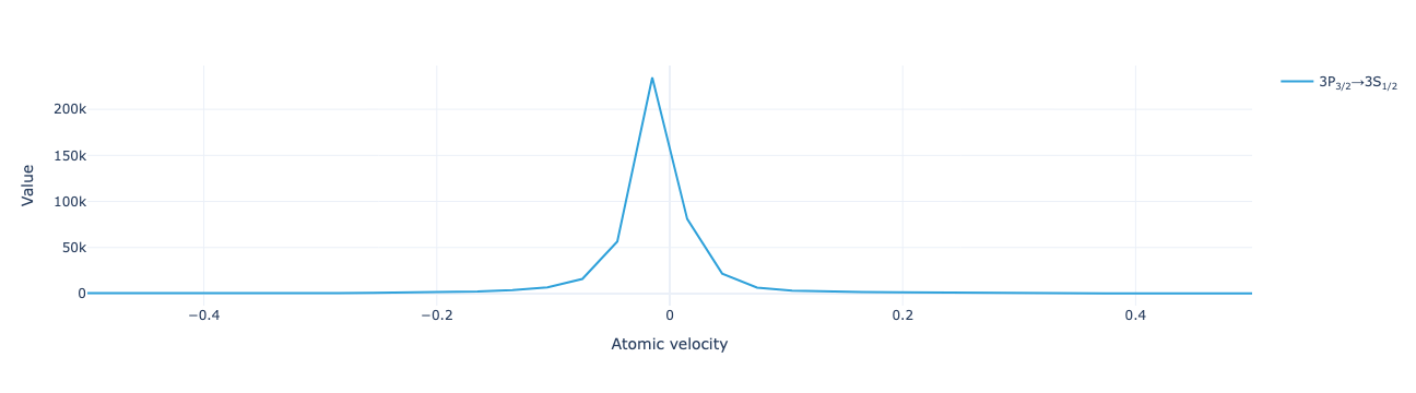
Plot the level population distribution:
model.level_population_distribution(sol).visualize()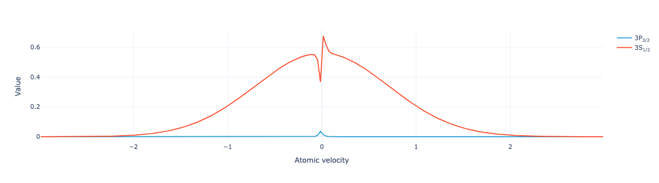
Adaptive refinement of velocity groups
Build a steady-state model with each velocity group contributing no more than 2% of the return flux:
model = lgs.adaptive_stationary_model(params, max_weight=0.02)Find the total flux for this model:
model.total_flux(params).item()13521.853828091767Find the density matrix. In this case the adaptive refinement has produced 82 velocity groups:
sol = model.solve(params)
sol
∅ ⛒ Atomic velocity(82) ⛒ Density matrix(374)
<xarray.DataArray (Atomic velocity: 82, Density matrix: 374)> Size: 245kB
array([[ 4.44509872e-04,  1.36091036e-04, -1.35996327e-04, ...,
         5.04360665e-08,  3.13451678e-10,  5.04876034e-11],
       [ 1.45887607e-02,  4.46721785e-03, -4.46295751e-03, ...,
         2.70911635e-06,  2.75753862e-08,  3.64921516e-09],
       [ 1.26044868e-02,  3.86768996e-03, -3.86086257e-03, ...,
         3.88703946e-06,  6.57920988e-08,  7.98942086e-09],
       ...,
       [ 1.24522695e-02,  3.87768725e-03, -3.86835956e-03, ...,
        -4.56188071e-06,  9.01968985e-08,  1.08025349e-08],
       [ 1.45004997e-02,  4.47569072e-03, -4.47010941e-03, ...,
        -2.97033838e-06,  3.30992815e-08,  4.28594841e-09],
       [ 4.43024154e-04,  1.36270775e-04, -1.36153854e-04, ...,
        -5.32867789e-08,  3.49646975e-10,  5.46598004e-11]],
      shape=(82, 374))
Coordinates:
  * Atomic velocity  (Atomic velocity) float64 656B -2.5 -1.5 -0.875 ... 1.5 2.5
* Density matrix (Density matrix) <U68 102kB 'ρ<sub>Re, (3S<sub>1/2</sub>...The flux distribution shows that this is a more detailed description of the system than the model with a greater number of evenly spaced velocity groups:
model.flux_distribution(sol).visualize(xaxis_range=(-.5, .5))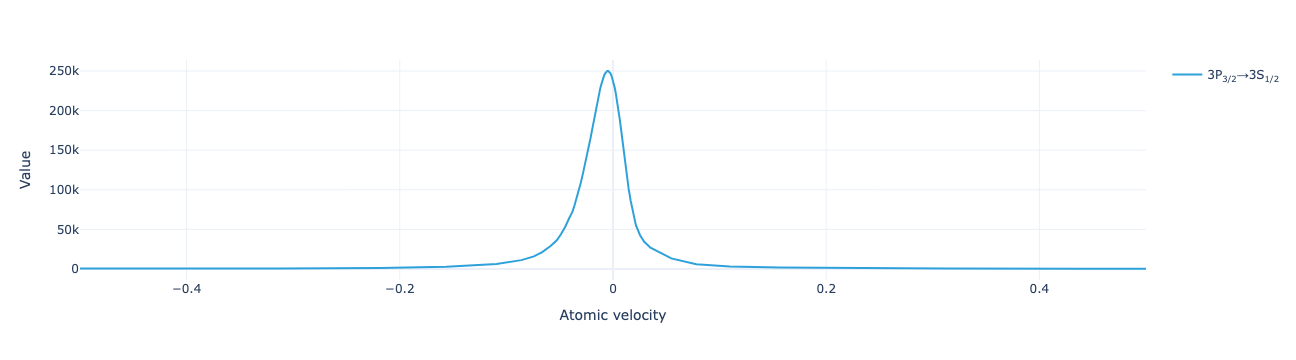
Dependence on system parameters
Find the steady-state density matrix for 10 different values of repump intensity, with the total pump + repump intensity held constant:
sol = model.solve([
    {'BFieldG': .5},
    {
        'IntensitySI1': np.linspace(0, 25, 10),
        'IntensitySI2': 50 - np.linspace(0, 25, 10)
    }
])
sol
IntensitySI1(10) ⛒ Atomic velocity(82) ⛒ Density matrix(374)
<xarray.DataArray (IntensitySI1: 10, Atomic velocity: 82, Density matrix: 374)> Size: 2MB
array([[[ 2.84741842e-04,  7.60632966e-05, -7.60110985e-05, ...,
          0.00000000e+00,  0.00000000e+00,  0.00000000e+00],
        [ 9.34061246e-03,  2.49835302e-03, -2.49584954e-03, ...,
          0.00000000e+00,  0.00000000e+00,  0.00000000e+00],
        [ 8.05861498e-03,  2.16697087e-03, -2.16267737e-03, ...,
          0.00000000e+00,  0.00000000e+00,  0.00000000e+00],
        ...,
        [ 7.96427298e-03,  2.17609075e-03, -2.17017686e-03, ...,
          0.00000000e+00,  0.00000000e+00,  0.00000000e+00],
        [ 9.28659916e-03,  2.50480549e-03, -2.50147362e-03, ...,
          0.00000000e+00,  0.00000000e+00,  0.00000000e+00],
        [ 2.83838071e-04,  7.61913869e-05, -7.61254749e-05, ...,
          0.00000000e+00,  0.00000000e+00,  0.00000000e+00]],

       [[ 4.01698906e-04,  1.20402788e-04, -1.20313939e-04, ...,
          4.17564068e-08,  2.59508023e-10,  3.09733262e-11],
        [ 1.31811455e-02,  3.95223864e-03, -3.94826757e-03, ...,
          2.24335803e-06,  2.28344071e-08,  2.24630961e-09],
        [ 1.13815087e-02,  3.42174937e-03, -3.41544293e-03, ...,
          3.22055406e-06,  5.45105782e-08,  4.92852730e-09],
...
         -6.30235065e-06,  1.24606708e-07,  3.15669222e-08],
        [ 2.04090178e-02,  6.60686901e-03, -6.60293236e-03, ...,
         -4.12235622e-06,  4.59360751e-08,  1.26554421e-08],
        [ 6.22589326e-04,  2.01194662e-04, -2.01123442e-04, ...,
         -7.40494824e-08,  4.85881154e-10,  1.63604212e-10]],

       [[ 6.43985708e-04,  2.08149758e-04, -2.08105532e-04, ...,
          7.04584838e-08,  4.37889509e-10,  1.61340275e-10],
        [ 2.11471524e-02,  6.83282173e-03, -6.83033178e-03, ...,
          3.77328809e-06,  3.84075560e-08,  1.14886043e-08],
        [ 1.83094768e-02,  5.91546057e-03, -5.91046723e-03, ...,
          5.37081808e-06,  9.09074025e-08,  2.48009332e-08],
        ...,
        [ 1.81826735e-02,  5.92391218e-03, -5.91694764e-03, ...,
         -6.34100470e-06,  1.25370996e-07,  3.36838857e-08],
        [ 2.10739198e-02,  6.84013860e-03, -6.83659003e-03, ...,
         -4.15204473e-06,  4.62669190e-08,  1.35143463e-08],
        [ 6.42757305e-04,  2.08306456e-04, -2.08244261e-04, ...,
         -7.46058793e-08,  4.89532153e-10,  1.74651106e-10]]],
      shape=(10, 82, 374))
Coordinates:
  * IntensitySI1     (IntensitySI1) float64 80B 0.0 2.778 5.556 ... 22.22 25.0
  * Atomic velocity  (Atomic velocity) float64 656B -2.5 -1.5 -0.875 ... 1.5 2.5
* Density matrix (Density matrix) <U68 102kB 'ρ<sub>Re, (3S<sub>1/2</sub>...Plot the total flux to show the optimal value of repump intensity for these conditions:
model.total_flux(sol).visualize()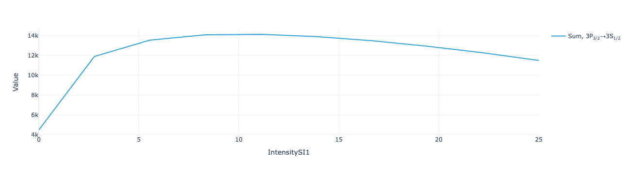
Create an animation of the flux distribution as the repump intensity is varied:
model.flux_distribution(sol).visualize(xaxis_range=(-.5, .5))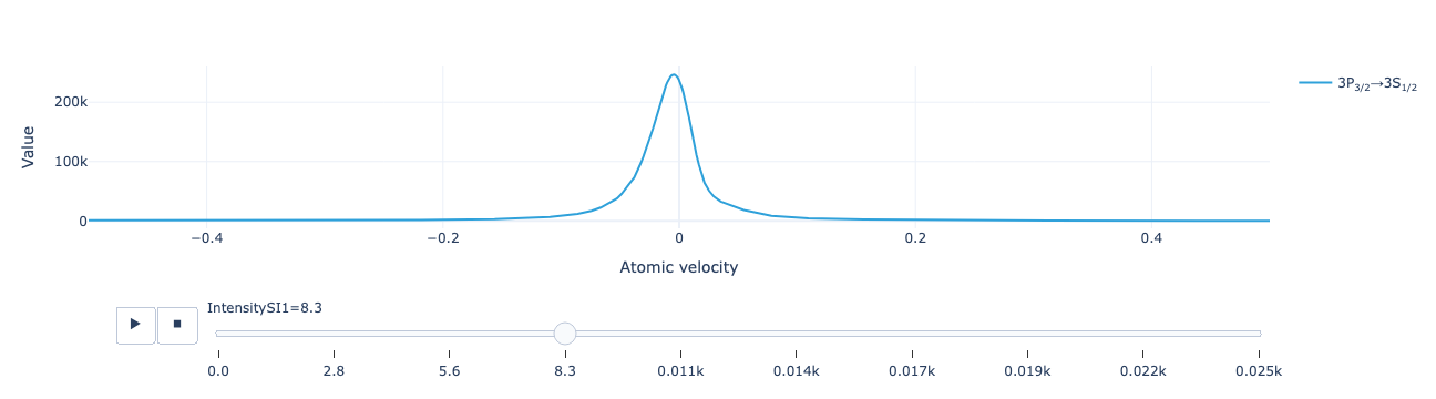
Animate the level population distribution as a function of repump intensity:
model.level_population_distribution(sol).visualize()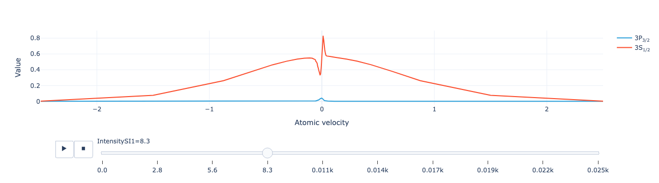
Transient dynamics
Transient dynamics from a laser pulse (Adams solver)
Build a dynamical model (InstationaryModel) using the velocity groups from the adaptively refined steady-state model:
lgs = LGSSystem(
    'NaD2_Repump',
    {
        'EllipticityDegrees1': 45.,
        'PolarizationAngleDegrees1': 0,
        'DetuningHz1': 1.0832e9,
        'LaserWidthHz1': 10.0e6,
        'EllipticityDegrees2': 45.,
        'PolarizationAngleDegrees2': 0,
        'DetuningHz2': -6.268e8,
        'LaserWidthHz2': 10.0e6,
        'MagneticZenithDegrees': 45.,
        'MagneticAzimuthDegrees': 45.,
        'SDampingCollisionRatePerS': 4081.63,
        'BeamTransitRatePerS': 131.944,
        'VccRatePerS': 28571.,
        'TemperatureK': 185.,
        'RecoilParameter': 1,
        'BFieldG': .5
    }
)
model = lgs.instationary_model(
vg=100,
T=1e-8,
num_values=100,
time_stepper=AdamsTimeStepper()
)params = {
'IntensitySI1': "5.*sin(1e6*t)**2",
'IntensitySI2': "46.*sin(1e6*t)**2",
}Solve for the density-matrix evolution. The solution contains the density matrix for each velocity group at 100 time values:
sol = model.solve(params)Plot the total flux as a function of time:
model.total_flux(sol).visualize()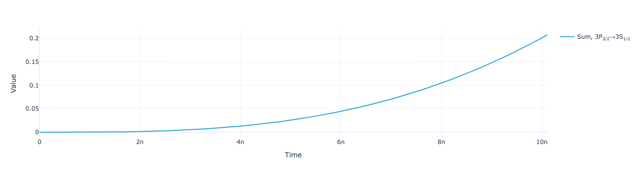
Animate the flux distribution as a function of time:
model.flux_distribution(sol).visualize()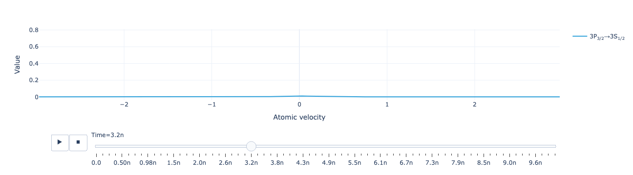
Animate the level population distribution:
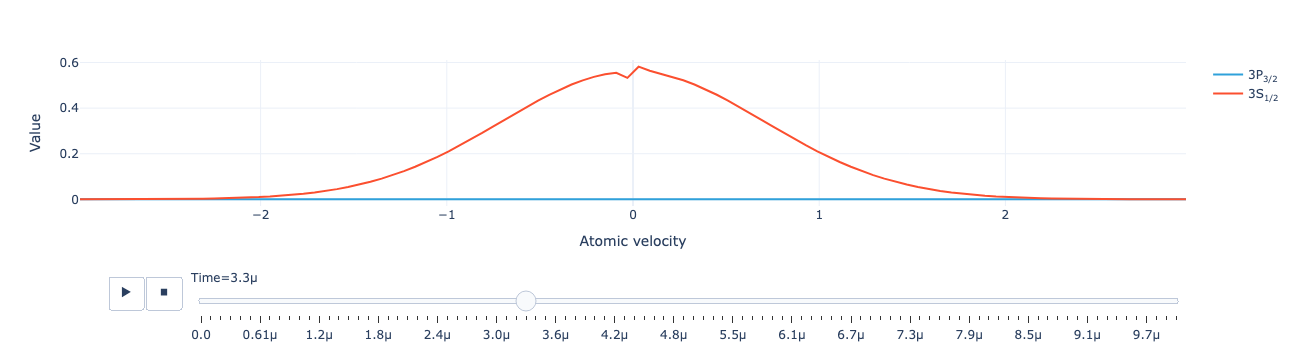
model.level_population_distribution(sol).visualize(xaxis_range=(-1, 1))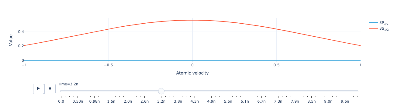
model.total_population(sol).visualize()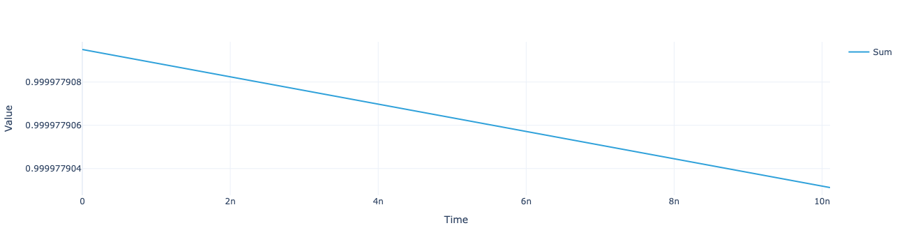
Transient dynamics from a laser pulse
Build a dynamical model (InstationaryModel) using the velocity groups from the adaptively refined steady-state model:
model = lgs.instationary_model(
    vg=model.data['velocity_groups'],
    T=1e-5,
    num_values=100
)
Set tolerances for the BDF solver:
pymor.basic.set_defaults({
    'pylgs.pymor.timestepping.cvode_solver_options.cvode_bdf_atol': 1e-6,
    'pylgs.pymor.timestepping.cvode_solver_options.cvode_bdf_rtol': 1e-4,
})
Solve for the density-matrix evolution. The solution contains the density matrix for each velocity group at 100 time values:
sol = model.solve(params)
sol
Time(57) ⛒ Atomic velocity(100) ⛒ Density matrix(374)
<xarray.DataArray (Time: 57, Atomic velocity: 100, Density matrix: 374)> Size: 17MB
array([[[ 6.27745202e-07,  0.00000000e+00,  0.00000000e+00, ...,
          0.00000000e+00,  0.00000000e+00,  0.00000000e+00],
        [ 8.93121976e-07,  0.00000000e+00,  0.00000000e+00, ...,
          0.00000000e+00,  0.00000000e+00,  0.00000000e+00],
        [ 1.26157506e-06,  0.00000000e+00,  0.00000000e+00, ...,
          0.00000000e+00,  0.00000000e+00,  0.00000000e+00],
        ...,
        [ 1.26157506e-06,  0.00000000e+00,  0.00000000e+00, ...,
          0.00000000e+00,  0.00000000e+00,  0.00000000e+00],
        [ 8.93121976e-07,  0.00000000e+00,  0.00000000e+00, ...,
          0.00000000e+00,  0.00000000e+00,  0.00000000e+00],
        [ 6.27745202e-07,  0.00000000e+00,  0.00000000e+00, ...,
          0.00000000e+00,  0.00000000e+00,  0.00000000e+00]],

       [[ 6.27745197e-07,  7.35444182e-29,  1.89679667e-27, ...,
          2.24369912e-12,  2.76626558e-14,  0.00000000e+00],
        [ 8.93121969e-07, -1.81177939e-24, -1.67989305e-24, ...,
          3.25650740e-12,  4.09585045e-14,  0.00000000e+00],
        [ 1.26157505e-06,  4.56553533e-27,  8.06669613e-27, ...,
          4.69451376e-12,  6.02589721e-14,  0.00000000e+00],
...
         -1.74172305e-10,  1.02687217e-12,  6.47153925e-14],
        [ 9.00346202e-07,  2.54237354e-09, -1.21374353e-08, ...,
         -1.20699853e-10,  6.96589237e-13,  4.44494037e-14],
        [ 6.32820094e-07,  1.78710610e-09, -8.52597131e-09, ...,
         -8.30812705e-11,  4.69569096e-13,  3.03412485e-14]],

       [[ 6.35124355e-07,  2.02808636e-09, -8.24736833e-09, ...,
          1.04971448e-10,  5.65104431e-13,  4.69083454e-14],
        [ 9.03628849e-07,  2.88741508e-09, -1.17394596e-08, ...,
          1.52357272e-10,  8.36726410e-13,  6.87259521e-14],
        [ 1.27642650e-06,  4.08107922e-09, -1.65906504e-08, ...,
          2.19637469e-10,  1.23102196e-12,  1.00060577e-13],
        ...,
        [ 1.27641608e-06,  3.94043083e-09, -1.66222729e-08, ...,
         -2.30397788e-10,  1.35456040e-12,  1.07562396e-13],
        [ 9.03621773e-07,  2.78995089e-09, -1.17610813e-08, ...,
         -1.59663688e-10,  9.18880282e-13,  7.37147109e-14],
        [ 6.35120598e-07,  1.96127505e-09, -8.26203415e-09, ...,
         -1.09901278e-10,  6.19415190e-13,  5.02063430e-14]]],
      shape=(57, 100, 374))
Coordinates:
  * Time             (Time) float64 456B 0.0 1.193e-08 ... 9.856e-06 1.001e-05
  * Atomic velocity  (Atomic velocity) float64 800B -2.97 -2.91 ... 2.91 2.97
* Density matrix (Density matrix) <U68 102kB 'ρ<sub>Re, (3S<sub>1/2</sub>...Plot the total flux as a function of time:
model.total_flux(sol).visualize()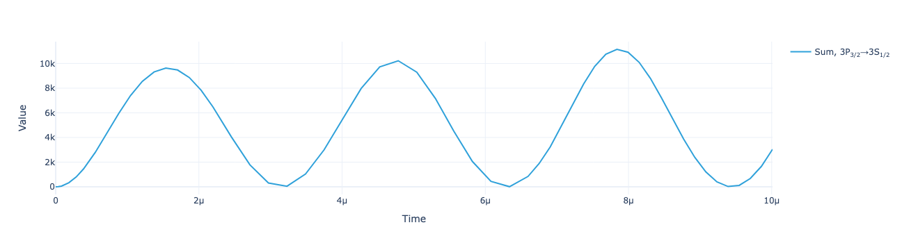
Animate the flux distribution as a function of time:
model.flux_distribution(sol).visualize()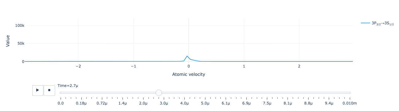
Animate the level population distribution:
model.level_population_distribution(sol).visualize(xaxis_range=(-1, 1))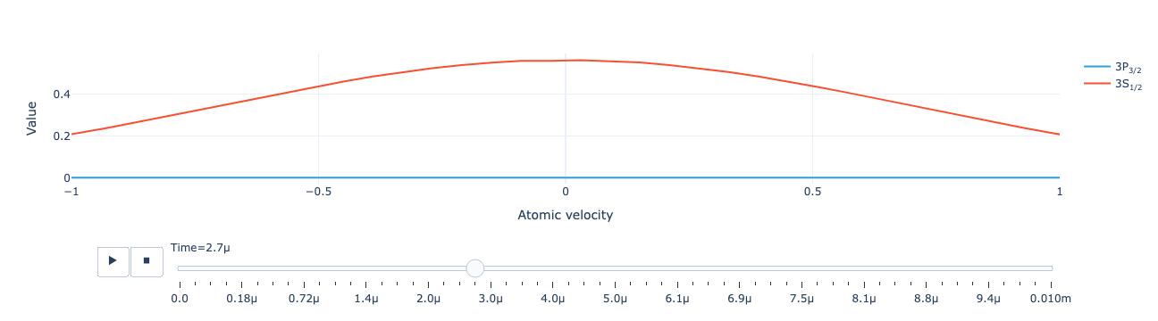
model.total_population(sol).visualize()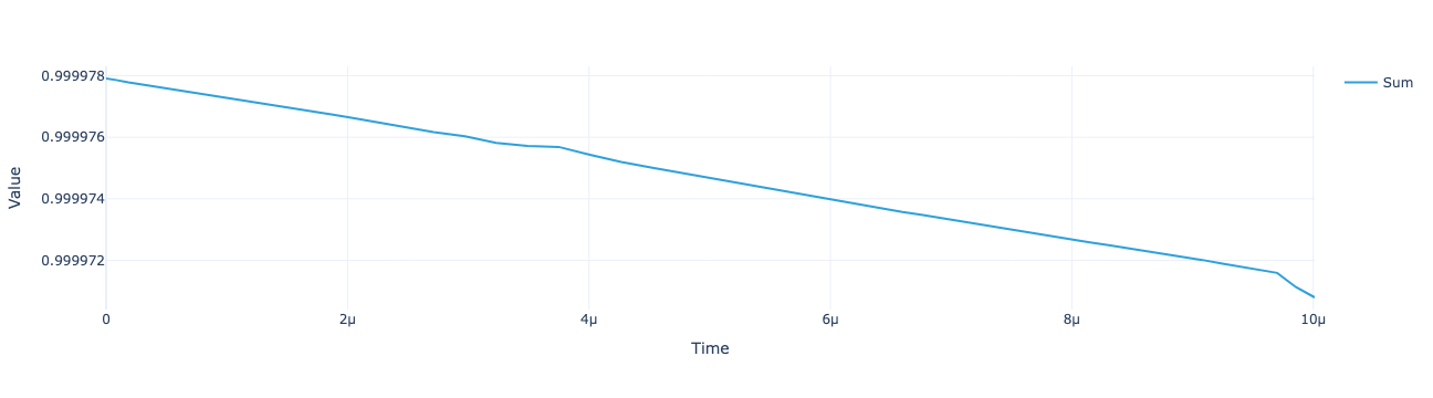
Transient dynamics with modulated laser intensity
Solve the InstationaryModel with sinusoidally modulated light intensity:
sol = model.solve({
    'IntensitySI1': "5.*sin(1e6*t)**2",
    'IntensitySI2': "46.*sin(1e6*t)**2",
})
The total flux as a function of time:
model.total_flux(sol).visualize()
The animated flux distribution:
model.flux_distribution(sol).visualize(xaxis_range=(-.25, .25))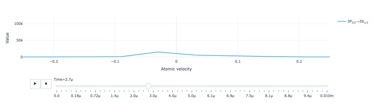
The animated level population distribution:
model.level_population_distribution(sol).visualize(xaxis_range=(-.25, .25))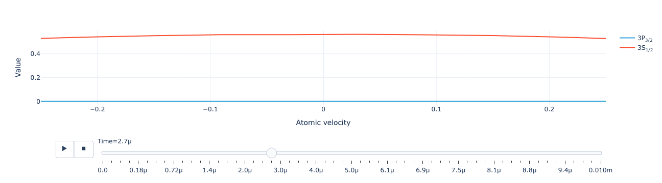
Periodic state of a modulated system
The StationaryFloquetModel solves for the periodic state of a modulated system after the transient dynamics have died out.
Build a stationary Floquet model for six Fourier harmonics of a system with sinusoidally modulated intensity:
model = lgs.stationary_floquet_model(
    {
        'IntensitySI1': "5.*sin(nu*t)**2",
        'IntensitySI2': "46.*sin(nu*t)**2"
    },
    time=np.linspace(0, 1e-5, 100),
    n_vector=6,
    vg=model.data['velocity_groups']
)
Define values for the modulation frequency and magnetic field:
mu = {'nu': 1e6}Solve for the periodic state. The solution contains 13 Fourier coefficients for each density-matrix element in each velocity group:
sol = model.solve(mu)
sol
∅ ⛒ Fourier coefficient(13) ⛒ Atomic velocity(100) ⛒ Density matrix(374)
<xarray.DataArray (Fourier coefficient: 13, Atomic velocity: 100,
                   Density matrix: 374)> Size: 8MB
array([[[-3.33369651e-12-2.47877648e-12j,
         -5.53433507e-12+2.76552152e-12j,
          6.95683437e-13+1.65700433e-13j, ...,
          1.91809872e-15-8.44185274e-16j,
          1.04261632e-17-3.65501220e-18j,
          1.47667554e-15-1.28265664e-16j],
        [-4.86099844e-12-3.55148666e-12j,
         -7.87301430e-12+4.09091277e-12j,
          9.67252287e-13+3.84130578e-13j, ...,
          2.75337483e-15-1.22273607e-15j,
          1.52726433e-17-5.41165723e-18j,
          2.16211906e-15-1.85490458e-16j],
        [-7.03984254e-12-5.05032620e-12j,
         -1.11194200e-11+6.00950444e-12j,
          1.33321190e-12+7.60456347e-13j, ...,
          3.92340423e-15-1.75885585e-15j,
          2.22173086e-17-7.96132736e-18j,
          3.14590176e-15-2.66516758e-16j],
        ...,
        [ 7.67471782e-12-4.41170965e-12j,
...
          3.14590177e-15+2.66516742e-16j],
        ...,
        [ 7.67472461e-12+4.41170889e-12j,
         -1.19787348e-11+1.45344441e-11j,
          3.76744779e-12+1.88575532e-11j, ...,
         -9.19847243e-15-2.65950797e-15j,
          5.39684785e-17+1.10517039e-17j,
          3.37720157e-15+2.78000299e-16j],
        [ 5.34129821e-12+3.10828377e-12j,
         -8.46855617e-12+1.01534257e-11j,
          2.65519277e-12+1.32179064e-11j, ...,
         -6.33506704e-15-1.83381395e-15j,
          3.63848299e-17+7.46343323e-18j,
          2.31593287e-15+1.93126838e-16j],
        [ 3.69197898e-12+2.17490151e-12j,
         -5.94445337e-12+7.04449712e-12j,
          1.85810764e-12+9.20113789e-12j, ...,
         -4.33463710e-15-1.25624124e-15j,
          2.43814837e-17+5.00960449e-18j,
          1.57835896e-15+1.33313848e-16j]]], shape=(13, 100, 374))
Coordinates:
  * Fourier coefficient  (Fourier coefficient) int64 104B -6 -5 -4 -3 ... 4 5 6
  * Atomic velocity      (Atomic velocity) float64 800B -2.97 -2.91 ... 2.97
* Density matrix (Density matrix) <U68 102kB 'ρ<sub>Re, (3S<sub>1/2</...The real and imaginary parts of the Fourier coefficients of the time-dependent return flux:
model.total_flux(sol).visualize()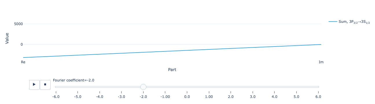
The total return flux reconstructed as a function of time:
model.reconstructed_total_flux(sol, mu).real.visualize()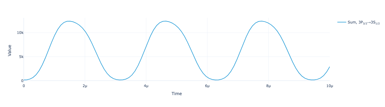
The level population distribution as a function of time:
model.level_population_distribution(model.reconstruct(sol, mu)).real.visualize()