from pylgs.all import *Sodium 589/569 nm LGS
A polychromatic sodium LGS excited by 589 nm and 569 nm light
LGSSystem loads the equations for an atomic system and sets values of parameters that are intended to be held fixed. Here we load a system that includes 589 nm and 569 nm pump light and fix all parameters except the detuning of 569 nm:
lgs = LGSSystem(
'Na589+569',
{
'IntensitySI1': 50., # Light intensity of the 589 nm laser in the mesosphere in W/m^2
'EllipticityDegrees1': 45., # Ellipticity of the 589 nm laser in degrees
'PolarizationAngleDegrees1': 0, # Polarization angle of the 589 nm laser in degrees
'DetuningHz1': 1.0832e9, # Detuning of the 589 nm laser in Hz
'LaserWidthHz1': 10.0e6, # Laser width of the 589 nm laser in Hz
'IntensitySI2': 100., # Light intensity of the 569 nm laser in the mesosphere in W/m^2
'EllipticityDegrees2': 45., # Ellipticity of the 569 nm laser in degrees
'PolarizationAngleDegrees2': 0, # Polarization angle of the 569 nm laser in degrees
# 'DetuningHz2': 1.1e8, # Detuning of the 569 nm laser in Hz
'LaserWidthHz2': 10.0e6, # Laser width of the 569 nm laser in Hz
'BFieldG': 0.5, # Mesospheric magnetic field strength in Gauss
'MagneticZenithDegrees': 45., # Zenith angle of the mesospheric magnetic field relative to the laser propagation direction in degrees
'MagneticAzimuthDegrees': 45., # Azimuth angle of the mesospheric magnetic field relative to the laser propagation direction in degrees
'SDampingCollisionRatePerS': 4081.63, # Spin damping collision rate in the mesosphere in s^-1
'BeamTransitRatePerS': 131.944, # Transit rate of atoms through the laser beam in s^-1
'VccRatePerS': 28571., # Velocity-changing collision rate in the mesosphere in s^-1
'TemperatureK': 185., # Temperature of the mesosphere in Kelvin
'RecoilParameter': 1. # Set to 1 to include recoil effects in the simulation, 0 to ignore them
}
)Print info about the atomic system:
LGSSystem.info('Na589+569')Atomic levels
\text{3S}_{\frac{1}{2}}, \text{3P}_{\frac{1}{2}}, \text{3P}_{\frac{3}{2}}, \text{4S}_{\frac{1}{2}}, \text{4P}_{\frac{3}{2}}, \text{4D}_{\frac{5}{2}}
Pump transitions
- \text{3S}_{\frac{1}{2}}\to \text{3P}_{\frac{3}{2}}
- \text{3P}_{\frac{3}{2}}\to \text{4D}_{\frac{5}{2}}
Transition wavelengths
- \text{3P}_{\frac{1}{2}}\to \text{3S}_{\frac{1}{2}}: 589.756 nm
- \text{3P}_{\frac{3}{2}}\to \text{3S}_{\frac{1}{2}}: 589.158 nm
- \text{4P}_{\frac{3}{2}}\to \text{3S}_{\frac{1}{2}}: 330.332 nm
- \text{4S}_{\frac{1}{2}}\to \text{3P}_{\frac{1}{2}}: 1138.46 nm
- \text{4S}_{\frac{1}{2}}\to \text{3P}_{\frac{3}{2}}: 1140.69 nm
- \text{4D}_{\frac{5}{2}}\to \text{3P}_{\frac{3}{2}}: 568.978 nm
- \text{4P}_{\frac{3}{2}}\to \text{4S}_{\frac{1}{2}}: 2206.24 nm
- \text{4D}_{\frac{5}{2}}\to \text{4P}_{\frac{3}{2}}: 2338.55 nm
Substructure
- Hyperfine structure included
- Zeeman structure included
- 80 total sublevels
Density matrix elements
- All populations included
- All Zeeman coherences (between same level and same F) included
- All hyperfine coherences (between same level and different F) neglected
- Optical coherences (between different levels) included for pump transitions only
- 1842 total density matrix elements
Input parameters
- BeamTransitRatePerS
- BFieldG
- MagneticAzimuthDegrees
- MagneticZenithDegrees
- RecoilParameter
- SDampingCollisionRatePerS
- TemperatureK
- VccRatePerS
- DetuningHz2
- DetuningHz1
- EllipticityDegrees2
- EllipticityDegrees1
- IntensitySI2
- IntensitySI1
- LaserWidthHz2
- LaserWidthHz1
- PolarizationAngleDegrees2
- PolarizationAngleDegrees1
A level diagram drawn to scale that neglects hyperfine and Zeeman structure:
LGSSystem.diagram('Na589+569', "Toy")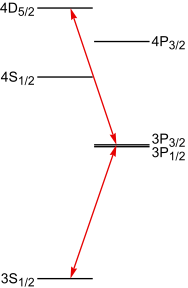
A level diagram, including hyperfine and Zeeman structure, not to scale:
LGSSystem.diagram('Na589+569', "NotToScale")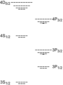
Create an adaptively refined model assuming a particular value of the 569 nm detuning by repeatedly subdividing velocity groups with the highest estimated local error until a specified relative global error estimate rtol is achieved. We return the results of the intermediate models so that we can illustrate the behavior as the the velocity groups are refined.
model, sol, inter = lgs.adaptive_stationary_model({'DetuningHz2': 1.1e8}, rtol=0.01, return_intermediate=True)Calculate the number of photons emitted in the mesosphere on each transition per atom per second per steradian in the return direction:
model.integrated_flux(sol).array<xarray.DataArray (Integral: 1, Transition: 8)> Size: 64B
array([[8.85249056e-02, 3.05768191e+02, 1.07218672e-01, 8.85250517e-02,
1.77050103e-01, 7.67127877e-01, 2.58884358e-01, 4.44426976e-01]])
Coordinates:
* Integral (Integral) int64 8B 1
* Transition (Transition) <U33 1kB '3P<sub>1/2</sub>→3S<sub>1/2</sub>' ......
Attributes:
long_name: Flux
units: photon/atom/s/srPlot the integrated flux as a bar plot:
model.integrated_flux(sol).visualize(log_x=True)Plot the distribution of return flux with respect to atomic velocity:
model.flux_distribution(sol).visualize(markers=True)Plotting on a log scale allows the velocity dependence of the weaker transitions to be easily seen:
model.flux_distribution(sol).visualize(log_y=True, markers=True)Plot the fractional populations of the 15 most populated atomic sublevels:
elems = sol.array.sum('Atomic velocity')
pops = elems.where(population_element(elems['Density matrix']), drop=True)
pops = pops.assign_coords({'Density matrix': [','.join(s.split(',')[1:4])[2:-1] for s in pops['Density matrix'].data]})
plotly_dataarray(pops.sortby(pops)[-15:], log_x=True)The global relative error estimate as a function of iteration:
p1 = plotly_dataarray(inter['global_err'].assign_attrs(units='', long_name='Global Error'), markers=True, log_y=True)
p1Plotting additional error estimates for each transition along with the global error estimate shows that, after about 8 iterations, the global error is a reasonable bound on the error for each transition:
p2 = plotly_dataarray(abs(inter['coarse_int'].diff('iteration')/inter['coarse_int'].isel(iteration=slice(1, None))).assign_coords(iteration=np.arange(1, inter['coarse_int'].sizes['iteration'])), markers=True, log_y=True)
p3 = plotly_dataarray(abs(inter['fine_int'].diff('iteration')/inter['fine_int'].isel(iteration=slice(1, None))).assign_coords(iteration=np.arange(1, inter['fine_int'].sizes['iteration'])), markers=True, log_y=True)
p1.add_traces(p2.data).add_traces(p3.data)Calculate integrated flux for each transition as a function of 569 nm detuning (will take several minutes):
results = []
deltas = np.linspace(-1e9, 1e9, 30)
for delta in deltas:
model, sol = lgs.adaptive_stationary_model({'DetuningHz2': delta}, rtol=.02)
results.append(model.integrated_flux(sol).array)
results = xr.concat(results, dim='delta').assign_coords(delta=deltas).squeeze()Plot the results for the weaker transitions:
plotly_dataarray(results, markers=True, yaxis_range=[0, 1])The flux for all transitions plotted on a log scale:
plotly_dataarray(results, log_y=True, markers=True)Calculate and plot the return flux with a finer detuning sweep around the maximum:
results = []
deltas = np.linspace(0, 2e8, 30)
for delta in deltas:
model, sol = lgs.adaptive_stationary_model({'DetuningHz2': delta}, rtol=.02)
results.append(model.integrated_flux(sol).array)
results = xr.concat(results, dim='delta').assign_coords(delta=deltas).squeeze()plotly_dataarray(results, markers=True, yaxis_range=[0, 1])